Download
1 / 82
820 likes | 970 Vues
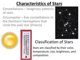
Unit 6:Life, Death and Characteristics of Stars. The Amazing Power of Starlight. Just by analyzing the light received from a star, astronomers can retrieve information about a star’s. Total energy output Surface temperature Radius Chemical composition Velocity relative to Earth

E N D
The Amazing Power of Starlight Just by analyzing the light received from a star, astronomers can retrieve information about a star’s • Total energy output • Surface temperature • Radius • Chemical composition • Velocity relative to Earth • Rotation period
Black Body Radiation (1) The light from a star is usually concentrated in a rather narrow range of wavelengths. The spectrum of a star’s light is approximately a thermal spectrum called a black body spectrum. A perfect black body emitter would not reflect any radiation. Thus the name “black body”.
The Color Index (1) The color of a star is measured by comparing its brightness in two different wavelength bands: The blue (B) band and the visual (V) band. We define B-band and V-band magnitudes just as we did before for total magnitudes (remember: a larger number indicates a fainter star). B band V band
The Color Index (2) We define the Color Index B – V (i.e., B magnitude – V magnitude). The bluer a star appears, the smaller the color index B – V. The hotter a star is, the smaller its color index B – V.
Light and Matter Spectra of stars are more complicated than pure blackbody spectra. characteristic lines, called absorption lines. To understand those lines, we need to understand atomic structure and the interactions between light and atoms.
Atomic Structure • An atom consists of an atomic nucleus (protons and neutrons) and a cloud of electrons surrounding it. • Almost all of the mass is contained in the nucleus, while almost all of the space is occupied by the electron cloud.
Atomic Density If you could fill a teaspoon just with material as dense as the matter in an atomic nucleus, it would weigh ~ 2 billion tons!!
Different Kinds of Atoms • The kind of atom depends on the number of protons in the nucleus. Different numbers of neutrons↔ different isotopes • Most abundant: Hydrogen (H), with one proton (+ 1 electron). • Next: Helium (He), with 2 protons (and 2 neutrons + 2 el.). Helium 4
Electron Orbits • Electron orbits in the electron cloud are restricted to very specific radii and energies. r3, E3 r2, E2 r1, E1 • These characteristic electron energies are different for each individual element.
Atomic Transitions • An electron can be kicked into a higher orbit when it absorbs a photon with exactly the right energy. Eph = E3 – E1 Eph = E4 – E1 Wrong energy • The photon is absorbed, and the electron is in an excited state. (Remember that Eph = h*f) • All other photons pass by the atom unabsorbed.
Kirchhoff’s Laws of Radiation (1) • A solid, liquid, or dense gas excited to emit light will radiate at all wavelengths and thus produce a continuous spectrum.
Kirchhoff’s Laws of Radiation (2) 2. A low-density gas excited to emit light will do so at specific wavelengths and thus produce an emission spectrum. Light excites electrons in atoms to higher energy states Transition back to lower states emits light at specific frequencies
Kirchhoff’s Laws of Radiation (3) 3. If light comprising a continuous spectrum passes through a cool, low-density gas, the result will be an absorption spectrum. Light excites electrons in atoms to higher energy states Frequencies corresponding to thetransition energies are absorbed from the continuous spectrum.
The Spectra of Stars Inner, dense layers of a star produce a continuous (blackbody) spectrum. Cooler surface layers absorb light at specific frequencies. => Spectra of stars are absorption spectra.
Analyzing Absorption Spectra • Each element produces a specific set of absorption (and emission) lines. • Comparing the relative strengths of these sets of lines, we can study the composition of gases. By far the most abundant elements in the Universe
Lines of Hydrogen Most prominent lines in many astronomical objects:Balmer lines of hydrogen
The Balmer Lines n = 1 n = 4 Transitions from 2nd to higher levels of hydrogen n = 5 n = 3 n = 2 Ha Hb Hg The only hydrogen lines in the visible wavelength range. 2nd to 3rd level = Ha (Balmer alpha line) 2nd to 4th level = Hb (Balmer beta line) …
Observations of the H-Alpha Line Emission nebula, dominated by the red Ha line.
Absorption Spectrum Dominated by Balmer Lines Modern spectra are usually recorded digitally and represented as plots of intensity vs. wavelength
The Balmer Thermometer Balmer line strength is sensitive to temperature: Most hydrogen atoms are ionized => weak Balmer lines Almost all hydrogen atoms in the ground state (electrons in the n = 1 orbit) => few transitions from n = 2 => weak Balmer lines
Measuring the Temperatures of Stars Comparing line strengths, we can measure a star’s surface temperature!
Spectral Classification of Stars (1) Different types of stars show different characteristic sets of absorption lines. Temperature
Spectral Classification of Stars (2) Mnemonics to remember the spectral sequence:
Stellar Spectra O B A F Surface temperature G K M
The Composition of Stars From the relative strength of absorption lines (carefully accounting for their temperature dependence), one can infer the composition of stars.
The Doppler Effect The light of a moving source is blue/red shifted by Dl/l0 = vr/c l0 = actual wavelength emitted by the source Dl = Wavelength change due to Doppler effect vr = radial velocity Blue Shift (to higher frequencies) Red Shift (to lower frequencies) vr
The Doppler Effect (2) The Doppler effect allows us to measure the source’s radial velocity. vr
The Doppler Effect (3) Take l0 of the Ha (Balmer alpha) line: l0 = 656 nm Assume, we observe a star’s spectrum with the Ha line at l = 658 nm. Then, Dl = 2 nm. We findDl/l0 = 0.003 = 3*10-3 Thus, vr/c = 0.003, or vr = 0.003*300,000 km/s = 900 km/s. The line is red shifted, so the star is receding from us with a radial velocity of 900 km/s.
Doppler Broadening In principle, line absorption should only affect a very unique wavelength. In reality, also slightly different wavelengths are absorbed. ↔ Lines have a finite width; we say: they are broadened. Blue shifted abs. Red shifted abs. One reason for broadening: The Doppler effect! vr Observer vr Atoms in random thermal motion
Line Broadening • Higher Temperatures • Higher thermal velocities broader lines Doppler Broadening is usually the most important broadening mechanism.
Distances to Stars d in parsec (pc) p in arc seconds __ 1 d = p Trigonometric Parallax: Star appears slightly shifted from different positions of the Earth on its orbit 1 pc = 3.26 LY The farther away the star is (larger d), the smaller the parallax angle p.
The Trigonometric Parallax Example: Nearest star, a Centauri, has a parallax of p = 0.76 arc seconds d = 1/p = 1.3 pc = 4.3 LY With ground-based telescopes, we can measure parallaxes p ≥ 0.02 arc sec => d ≤ 50 pc This method does not work for stars farther away than 50 pc.
Proper Motion In addition to the periodic back-and-forth motion related to the trigonometric parallax, nearby stars also show continuous motions across the sky. These are related to the actual motion of the stars throughout the Milky Way, and are called proper motion.
Intrinsic Brightness/ Absolute Magnitude The more distant a light source is, the fainter it appears.
Intrinsic Brightness / Absolute Magnitude (2) More quantitatively: The flux received from the light is proportional to its intrinsic brightness or luminosity (L) and inversely proportional to the square of the distance (d): L __ F ~ d2 Star A Star B Earth Both stars may appear equally bright, although star A is intrinsically much brighter than star B.
Distance and Intrinsic Brightness Example: Recall that: Betelgeuse App. Magn. mV = 0.41 Rigel For a magnitude difference of 0.41 – 0.14 = 0.27, we find an intensity ratio of (2.512)0.27 = 1.28 App. Magn. mV = 0.14
Distance and Intrinsic Brightness (2) Rigel is appears 1.28 times brighter than Betelgeuse, Betelgeuse But Rigel is 1.6 times further away than Betelgeuse Thus, Rigel is actually (intrinsically) 1.28*(1.6)2 = 3.3 times brighter than Betelgeuse. Rigel
Absolute Magnitude To characterize a star’s intrinsic brightness, define Absolute Magnitude (MV): Absolute Magnitude = Magnitude that a star would have if it were at a distance of 10 pc.
Absolute Magnitude (2) Back to our example of Betelgeuse and Rigel: Betelgeuse Rigel Difference in absolute magnitudes: 6.8 – 5.5 = 1.3 => Luminosity ratio = (2.512)1.3 = 3.3
The Distance Modulus If we know a star’s absolute magnitude, we can infer its distance by comparing absolute and apparent magnitudes: Distance Modulus = mV – MV = -5 + 5 log10(d [pc]) Distance in units of parsec Equivalent: d = 10(mV – MV + 5)/5 pc
The Size (Radius) of a Star We already know: flux increases with surface temperature (~ T4); hotter stars are brighter. But brightness also increases with size: Star B will be brighter than star A. A B Absolute brightness is proportional to radius squared, L ~ R2. Quantitatively: L = 4 p R2s T4 Surface flux due to a blackbody spectrum Surface area of the star
Example: Star Radii Polaris has just about the same spectral type (and thus surface temperature) as our sun, but it is 10,000 times brighter than our sun. Thus, Polaris is 100 times larger than the sun. This causes its luminosity to be 1002 = 10,000 times more than our sun’s.
Organizing the Family of Stars: The Hertzsprung-Russell Diagram We know: Stars have different temperatures, different luminosities, and different sizes. To bring some order into that zoo of different types of stars: organize them in a diagram of Luminosity Temperature (or spectral type) versus Absolute mag. Hertzsprung-Russell Diagram Luminosity or Temperature Spectral type: O B A F G K M
The Hertzsprung-Russell Diagram Most stars are found along the Main Sequence
The Hertzsprung-Russell Diagram (2) Same temperature, but much brighter than MS stars Must be much larger Stars spend most of their active life time on the Main Sequence (MS). Giant Stars Same temp., but fainter → Dwarfs
The Radii of Stars in the Hertzsprung-Russell Diagram Rigel Betelgeuse 10,000 times the sun’s radius Polaris 100 times the sun’s radius Sun As large as the sun 100 times smaller than the sun
Luminosity Classes Ia Bright Supergiants Ia Ib Ib Supergiants II II Bright Giants III III Giants IV Subgiants IV V V Main-Sequence Stars
Example Luminosity Classes • Our Sun: G2 star on the Main Sequence:G2V • Polaris: G2 star with Supergiant luminosity: G2Ib
Spectral Lines of Giants Pressure and density in the atmospheres of giants are lower than in main sequence stars. => Absorption lines in spectra of giants and supergiants are narrower than in main sequence stars => From the line widths, we can estimate the size and luminosity of a star. Distance estimate (spectroscopic parallax)