Download
1 / 19
210 likes | 379 Vues
Lecture 4 Sampling and Estimation. Dr Peter Wheale. Sampling. To make inferences about the parameters of a population, we will use a sample A simple random sample is one where every population member has an equal chance of being selected

E N D
Lecture 4Sampling and Estimation Dr Peter Wheale
Sampling • To make inferences about the parameters of a population, we will use a sample • A simple random sample is one where every population member has an equal chance of being selected • A sampling distribution is the distribution of sample statistics for repeated samples of size n • Sampling error is the difference between a sample statistic and true population parameter
Use of n – sample size versus N – population size • Data set of a stock’s returns over time: • 12%, 25%, 34%, 15% , 19%, 44%, 54%, 33%, 22%, 28%, 17%, 24% • µ = 12+25+34+15+19+44+54+33+22+28+17+24 / 12 =27.25% x = 25+34+19+54+17 / 5 = 29.8% In the above calculations the population size, N, is 12, and the sample size, n, is 5. All interval and ratio data sets have an arithmetic mean. • The population mean and sample mean are both examples of arithmetic means – the most common measure of central tendency. • The arithmetic mean is unique and the sum of the deviations of each observation in the data set from the mean is zero. • The sampling error of the mean = 29.8% - 27.25% = 2.55.
Stratified Random Sampling 1. Create subgroups from population based on important characteristics, e.g. identify bonds according to: callable, ratings, maturity, coupon 2. Select samples from each subgroup in proportion to the size of the subgroup Used to construct bond portfolios to match a bond index or to construct a sample that has certain characteristics in common with the underlying population
Time-Series vs. Cross-Sectional Time-series data e.g. Monthly prices for IBM stock for 5 years Cross-sectional data e.g. Returns on all health care stocks last month
Central Limit Theorem • For any population with mean µ and variance σ2, as the size of a random sample gets large, the distribution of sample means approaches a normal dist. with mean µ and variance σ2 • Allows us to make inferences about and construct confidence intervals for population means based on sample means
Semivariance and CV • Semivariance is calculated by only including those observations that fall below the mean ion the calculation. • Sometimes described as “downside risk” with respect to investments. • Useful for skewed distributions, as it provides additional information that the variance does not. • Target semivariance is similar but based on observations below a certain value, e.g values below a return of 5%. • Coefficient of Variation (CV) = standard deviation of x • average value of x • X can stand for investments for example ; CV measures the risk (variability) per unit of expected return (mean).
CV Example • CV calculation: = standard deviation of x • average value of x • Example: Suppose you wish to calculate the CV for two investments, the monthly return on British T-Bills and the monthly return for the S&P 500, where: mean monthly return on T-Bills is 0.25% with SD of 0.36%, and the mean monthly return for the S&P 500 is 1.09%, with a SD of 7.30%. • CV (T-Bills) = 0.36/0.25 = 1.44 • CV (S&P 500) = 7.30/1.09 = 6.70 • Interpretation: is the variation per unit of return, indicating that these results indicate that there is less dispersion (risk) per unit of monthly returns for T-Bills than there is for the S&P 500, i.e. 1.44 vs 6.70.
Standard Error of the Sample Mean Standard error of sample mean is the standard deviation of the distribution of sample means. • When the population σ is known: • When the population σ is unknown:
Standard Error of the Sample Mean Example: The mean P/E for a sample of 41 firms is 19.0, and the standard deviation of the population is 6.6. What is the standard error of the sample mean? Interpretation: For samples of size n = 41, the distribution of the sample means would have a mean of 19.0 and a standard error of 1.03.
Point Estimate and Confidence Interval Example: The mean P/E for a sample of 41 firms is 19.0, the standard error of the sample mean is 1.03, and the population is normal Point estimate of mean is 19.0 90% confidence interval is 19 +/- 1.65 (1.03) 17.3 < mean < 20.7 95% confidence interval is 19 +/- 1.96 (1.03) 17.0 < mean < 21.0
Confidence Interval: Normal Distribution Confidence interval: a range of values around an expected outcome within which we expect the actual outcome to occur some specified percent of the time.
Properties of Normal Distribution • Completely described by mean and variance • Symmetric about the mean (skewness = 0) • Kurtosis (a measure of peakedness) = 3 • Linear combination of normally distributed random variables is also normally distributed • Probabilities decrease further from the mean, but the tails go on forever
Kurtosis - peakedness • Kurtosis is a measure of the degree to which a distribution is more or less “peaked” than a normal distribution. Leptokurtic describes a distribution that is more peaked than a normal distribution – it will have more returns clustered around the mean and large deviations from the mean - and platykurtic describes a distribution that is less peaked (flatter than a normal distribution) – having a broader spread of deviations from the mean. • Skewness and kurtosis are important in for risk management because model predictions need to take account of the distribution of returns in the tails of the distribution, which is where the risk lies.
Measures of Sample Skew and Kurtosis • Sample skewness is equal to the sum of the cubed deviations from the mean divided by the cubed standard deviation and by the number of observations. • A left skewed distribution is negative and a right skewed distribution is positive. • Sample kurtosis is measured as above, but using deviations raised to the fourth power. • Interpretation of kurtosis: calculations are compared to the value for a normal distribution curve, which is 3. • Excess kurtosis = sample kurtosis – 3.
Confidence Interval: Normal Distribution • Example: The mean annual return (normally distributed) on a portfolio over many years is 11%, and the standard deviation of returns is 8%. A 95% confidence interval on next year’s return is 11% + (1.96)(8%) = –4.7% to 26.7%
Desirable Estimator Properties 1. Unbiased- expected value equal to parameter 2. Efficient- sampling distribution has smallest variance of all unbiased estimators 3. Consistent– larger sample → better estimator Standard error of estimate decreases with larger sample size
Student’s t-Distribution and Degrees of Freedom Properties of Student’s t-Distribution • Symmetrical (bell shaped) • Less peaked and fatter tails than a normal distribution • Defined by single parameter, degrees of freedom (df), where df = n – 1 • As df increase, t-distribution approaches normal distribution
t-Distribution The figure below shows the shape of the t-distribution with different degrees of freedom.