Download
1 / 26
260 likes | 377 Vues
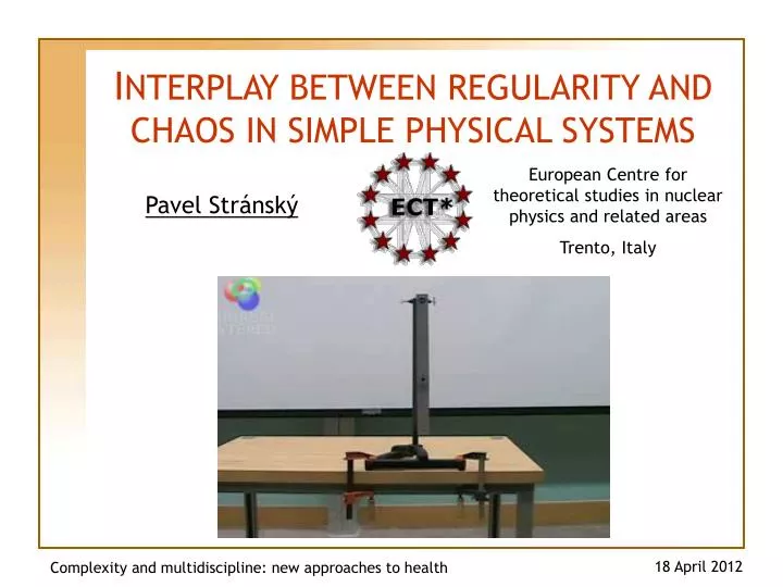
I NTERPLAY BETWEEN REGULARITY AND CHAOS IN SIMPLE PHYSICAL SYSTEMS. European Centre for theoretical studies in nuclear physics and related areas Trento, Italy. Pavel Str ánský. 18 April 2012. Complexity and multidiscipline: new approaches to health. Physics of the 1 st kind: CODING

E N D
INTERPLAY BETWEEN REGULARITY AND CHAOS IN SIMPLE PHYSICAL SYSTEMS European Centre for theoretical studies in nuclear physics and related areas Trento, Italy Pavel Stránský 18 April 2012 Complexity and multidiscipline: new approaches to health
Physics of the 1st kind: CODING Complex behaviour →Simple equations Physics of the 2nd kind: DECODING Simple equations → Complex behaviour
Hamiltonian 1.Classical physics It describes (for example): Motion of a star around a galactic centre, assuming the motion is restricted to a plane (Hénon-Heiles model) Collective motion of an atomicnucleus (Bohr model) • 2. Quantum physics
1. Classical chaos Trajectories (solutions of the equations of motion) y x
chaotic case – “fog” (hypersensitivity of the motion on the initial conditions) Section at y = 0 vx ordered case – “circles” x 1. Classical chaos We plot a point every time when a trajectory crosses a given line (y = 0) Trajectories (solutions of the equations of motion) vx y x Poincaré sections Coexistence of quasiperiodic (ordered) and chaotic types of motion
chaotic case – “fog” (hypersensitivity of the motion on the initial conditions) Section at y = 0 vx ordered case – “circles” x 1. Classical chaos We plot a point every time when a trajectory crosses a given line (y = 0) Trajectories (solutions of the equations of motion) vx y x Phase space 4D space comprising coordinates and velocities Poincaré sections Coexistence of quasiperiodic (ordered) and chaotic types of motion
vx x 1. Classical chaos Fraction of regularity Measure of classical chaos Surface of the section covered with regular trajectories Total kinematically accessible surface of the section REGULARarea CHAOTICarea freg=0.611
1. Classical chaos Complete map of classical chaos Totally regular limits Veins of regularity chaotic Phase transition regular control parameter Highly complex behaviour encoded in a simple equation P. Stránský, P. Hruška, P. Cejnar, Phys. Rev. E79 (2009), 046202
2. Quantum chaos Discrete energy spectrum Spectral density: smooth part oscillating part given by the volume of the classical phase space Gutzwiller formula (the sum of all classical periodic trajectories and their repetitions) The oscillating part of the spectral density can give relevant information about quantum chaos (related to the classical trajectories) Unfolding: A transformation of the spectrum that removes the smooth part of the level density Note: Improved unfolding procedure using the Empirical Mode Decomposition method in: I. Morales et al., Phys. Rev.E84, 016203 (2011)
2. Quantum chaos Spectral statistics Nearest-neighbor spacing distribution Wigner Poisson P(s) s REGULAR system CHAOTIC system distribution parameter w Brody - Artificial interpolationbetween Poisson andGOEdistribution - Measure of chaoticity of quantum systems
2. Quantum chaos Quantum chaos - examples Billiards They are also extensively studied experimentally Schrödingerequation: (for wave function) Helmholtz equation: (for intensity of el. field)
2. Quantum chaos Quantum chaos - applications Riemann zfunction: Prime numbers Riemann hypothesis: All points z(s)=0in the complex plane lieon the line s=½+iy (except trivial zeros on the real exis s=–2,–4,–6,…) GUE Zeros ofzfunction
2. Quantum chaos Quantum chaos - applications GOE Correlation matrix of the human EEG signal P. Šeba, Phys. Rev. Lett. 91 (2003), 198104
2. Quantum chaos Ubiquitous in the nature (many time signals or space characteristics of complex systems have 1/f power spectrum) 1/f noise - Fourier transformation of the time series constructed from energy levels fluctuations dn = 0 dk d4 Power spectrum d3 k d2 d1 = 0 a= 2 a= 2 a= 1 CHAOTIC system REGULAR system a= 1 Direct comparison of 3 measures of chaos A. Relañoet al., Phys. Rev. Lett. 89, 244102 (2002) E. Faleiro et al., Phys. Rev. Lett. 93, 244101 (2004) J. M. G. Gómez et al., Phys. Rev. Lett. 94, 084101 (2005)
regular regular chaotic 2. Quantum chaos Peres lattices A tool for visualising quantum chaos (an analogue of Poincaré sections) Lattice: energy Eiversus the mean value of a (nearly) arbitrary operator P partly ordered, partly disordered lattice always ordered for any operator P Integrable nonintegrable B = 0 B = 0.445 <P> <P> E E A. Peres, Phys. Rev. Lett.53, 1711 (1984)
2. Quantum chaos Peres lattices in GCM Small perturbationaffects only a localized part of the lattice (The place of strong level interaction) B = 0 B = 0.005 B = 0.05 B = 0.24 Narrow band due to ergodicity <L2> Peres lattices for two different operators Remnants of regularity <H’> E Integrable Increasing perturbation Empire of chaos P. Stránský, P. Hruška, P. Cejnar, Phys. Rev. E79 (2009), 066201
<L2> Zoom into the sea of levels E 2. Quantum chaos Dependenceon the classicality parameter Dependence of the Brody parameter on energy
2. Quantum chaos Classical and quantum measures - comparison B= 1.09 B= 0.24 Classical measure Quantum measure (Brody)
2. Quantum chaos 1/f noise Mixed dynamics A = 0.25 Calculation of a: a - 1 Each point –averaging over 32 successive sets of 64 levels in an energy window 1 - w regularity freg E
Appendix Fourier transform Fourier basis Signal Fourier transform calculates an “overlap” between the signal and a given basis How to construct a signal with the 1/f noise power spectrum? (reverse engineering) … 1. Interplay of many basic stationary modes
Appendix 2. sin exp x • Features: • A very simple analytical prescription • An Intrinsic Mode Function • (one single frequency at any time)
Enjoy the last slide! Thank you for your attention Summary • Simple toy models can serve as a theoretical laboratory useful to understand and master complex behaviour. • Methods of classical and quantum chaos can be applied to study more sophisticated models or to analyze signals that even originate in different sciences http://www-ucjf.troja.mff.cuni.cz/~geometric http://www.pavelstransky.cz