Download
1 / 46
780 likes | 2.23k Vues
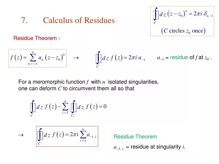
7. Calculus of Residues. Residue Theorem :. a 1 = residue of f at z 0. . For a meromorphic function f with n isolated singularities, one can deform C to circumvent them all so that. . Residue Theorem. a 1, i = residue at singularity i. Computing Residues.

E N D
7. Calculus of Residues Residue Theorem : a1 = residue of fat z0 . For a meromorphic functionf with nisolated singularities, one can deform C to circumvent them all so that Residue Theorem a1, i = residue at singularity i.
Computing Residues If f has a simple pole at z0 , simple poles If f has a pole of ordermat z0 , poles of orderm
Example 11.7.1. Computing Residues Some examples : Mathematica
Alternatively, z = 0 is a pole of 2nd order : Mathematica
Cauchy Principal Value Simple pole on path: Path: a b on real axis. Simple pole at x = x0. Eg. At x0, integral diverges as But the divergence cancels out if the pole is approached from both sides in a limiting process. Mathematica Cauchy principal value of a real integral with a simple pole at x0is defined as Caution: The real part of such integral is often defined by its Cauchy principal value. However, the integral itself is actually not convergent. For example, the value of the limit changes if we use different values of for different sides of x0.
Contour Integral & Cauchy Principal Value Contour C = ( ) + C (x0) + ( + ) + C. zj= poles inside C (excluding x0 ) Mathematica Contribution of a pole is halved if it lies on the contour.
Pole Expansion of Meromorphic Functions • Expansion of f about • A regular point Taylor series. • A pole Laurent series. • All simple poles (Mittag-Leffler) pole expansion.
Mittag-Leffler Theorem Let fbe meromorphic with simple poles at zj 0, (with residuebj) ;j = 1,..., M. If for large |z| , then Proof : Consider where CN is a circle centered at w=0, of radius RN, that encloses the 1stN poles of f closest to w=0. ForRN , QED
Example 11.7.3.Pole Expansion of tan z poles at Let
Example 11.7.4.Pole Expansion of cot z has at z = 0 with residue has poles at Let Similarly
Counting Poles & Zeros Let z0 be either a pole or zero of f (z). Set where g is regular at z0. if only zero or pole enclosed by C isz0. Nf = Sum of the orders of zeros of fenclosed by C. Pf = Sum of the orders of poles of fenclosed by C.
Rouche’s Theorem If f (z) &g(z) are analytic in the region R bounded by C and | f (z) | > | g(z) | on C, then f (z) & f (z) + g(z) have the same number of zeros in R. Cx = change of x going around C once. f (z) &g(z) are analytic Proof :
Example 11.7.5. Counting Zeros Let . Find NFfor To find NFfor , let with so that on C : |z| = 1 i.e., To find NFfor , let with so that on C : |z| = 3
Product Expansion of Entire Functions f (z) is an entire function if it is analytic for all finite z. Letf (z) be an entire function. Then is meromorphic (analytic except for poles for all finite z). Poles of F are zeros of f. If the M zeros, zj , of f are all simple (of order 1), then zjare simple poles of F with so that
Ex.11.7.5 Likewise Gamma function
8. Evaluation of Definite Integrals Trigonometric Integrals, Range (0,2) f= rational function & finite everywhere Set C = unit circle at z = 0. zj= poles inside C
Example 11.8.1.Integral of cos in Denominator inside outside C Poles at
Example 11.8.2.Another Trigonometric Integral Only poles at 0 & ½ are inside C.
Integrals, Range (, ) fis meromorphic in upper half z-plane, where C = Cx + CR R zjin upper plane Since (see next page for proof ) on upper plane Obviously, one can also close the contour in the lower half plane. zjin upper plane
on arc from 1 2 Proof : CR R 2 1 QED
Example 11.8.3. Integral of Meromorphic Function i i Poles are at . But only z+ is inside C. Alternatively
Integral with Complex Exponentials a > 0 & real. fanalytic in upper plane, where In upper plane, y > 0 R Jordan’s lemma zj= poles of f in upper plane
Example 11.8.4. Oscillatory Integral Poles are at Only z+is in upper plane with
Another Integration TechniqueExample 11.8.6. Evaluation on a Circular Sector Poles are at forj = 0,1,2 Branch cut On C , Set &
On Cr , On C,
Avoidance of Branch PointsExample 11.8.7. Integral Containing Logarithm Poles are at forj = 0,1,2 Branch cut On C , Set
On Cr , Branch cut On C, Ex.11.8.6
Exploiting Branch CutsExample 11.8.8. Using a Branch Cut i Branch cut i On C , On C+ ,
i Branch cut i On Cr , On C ,
i Branch cut i Poles are at
Example 11.8.9. Introducing a Branch Point Ex.11.8.6-7 evaluated 1st , then use it to get with a contour that avoids the branch cut. Here, we pretend to evaluate using a branch cut. But ends up with .
On C , On C+ ,
On Cr , On C ,
forj = 0,1,2 Poles are at
Exploiting PeriodicityExample 11.8.10. Integrand Periodic on Imaginary Axis i + R i R i sinh i n = 0 but x = 0 is not a pole since R R 0 n = integers since sinh xis odd On C / , &
9. Evaluation of Sums is meromorphic with simple poles at can be used to evaluate series. Consider where f is meromorphic with poles at zj.
Example 11.9.1.Evaluating a Sum a integer Poles of at with
Other Sum Formulae
Example 11.9.2. Another Sum has poles at z = 0, 1. has 2nd order poles at z = 0, 1. Mathematica
10. Miscellaneous Topics Schwarz reflection principle : If f (z) is analytic over region Rwith R x-axis , and f (x) is real, then Proof : For any f (x) is real f (n) (x) is real .
Mapping can be considered as a mapping Example Dotted circle = unit circle Mathematica