Download
1 / 58
580 likes | 647 Vues
Learning to Search. Henry Kautz University of Washington joint work with Dimitri Achlioptas, Carla Gomes, Eric Horvitz, Don Patterson, Yongshao Ruan, Bart Selman CORE – MSR, Cornell, UW. Speedup Learning. Machine learning historically considered Learning to classify objects

E N D
Learning to Search Henry Kautz University of Washington joint work with Dimitri Achlioptas, Carla Gomes, Eric Horvitz, Don Patterson, Yongshao Ruan, Bart Selman CORE – MSR, Cornell, UW
Speedup Learning • Machine learning historically considered • Learning to classify objects • Learning to search or reason more efficiently • Speedup Learning • Speedup learning disappeared in mid-90’s • Last workshop in 1993 • Last thesis 1998 • What happened? • It failed. • It succeeded. • Everyone got busy doing something else.
It failed. • Explanation based learning • Examine structure of proof trees • Explain why choices were good or bad (wasteful) • Generalize to create new control rules • At best, mild speedup (50%) • Could even degrade performance • Underlying search engines very weak • Etzioni (1993) – simple static analysis of next-state operators yielded as good performance as EBL
It succeeded. • EBL without generalization • Memoization • No-good learning • SAT: clause learning • Integrates clausal resolution with DPLL • Huge win in practice! • Clause-learning proofs can be exponentially smaller than best DPLL (tree shaped) proof • Chaff (Malik et al 2001) • 1,000,000 variable VLSI verification problems
Everyone got busy. • The something else: reinforcement learning. • Learn about the world while acting in the world • Don’t reason or classify, just make decisions • What isn’t RL?
Another path • Predictive control of search • Learn statistical model of behavior of a problem solver on a problem distribution • Use the model as part of a control strategy to improve the future performance of the solver • Synthesis of ideas from • Phase transition phenomena in problem distributions • Decision-theoretic control of reasoning • Bayesian modeling
control / policy dynamic features resource allocation / reformulation Big Picture runtime Solver Problem Instances Learning / Analysis static features Predictive Model
Case Study 1: Beyond 4.25 runtime Solver Problem Instances Learning / Analysis static features Predictive Model
Phase transitions & problem hardness • Large and growing literature on random problem distributions • Peak in problem hardness associated with critical value of some underlying parameter • 3-SAT: clause/variable ratio = 4.25 • Using measured parameter to predict hardness of a particular instance problematic! • Random distribution must be a good model of actual domain of concern • Recent progress on more realistic random distributions...
Quasigroup Completion Problem (QCP) • NP-Complete • Has structure is similar to that of real-world problems - tournament scheduling,classroom assignment, fiber optic routing, experiment design, ... • Can generate hard guaranteed SAT instances (2000)
Complexity Graph 20% 20% 42% 42% 50% 50% Phase Transition Critically constrained area Underconstrained area Overconstrained area Phase transition Almost all solvable area Almost all unsolvable area Fraction of unsolvable cases Fraction of pre-assignment
Walksat Order 30, 33, 36 Easy-Hard-Easy pattern in local search Computational Cost Underconstrained area “Over” constrained area % holes
Are we ready to predict run times? • Problem: high variance log scale
Rectangular Pattern Aligned Pattern Balanced Pattern Tractable Very hard Deep structural features Hardness is also controlled by structure of constraints, not just the fraction of holes
Random versus balanced Balanced Random
Random versus balanced Balanced Random
Random vs. balanced (log scale) Balanced Random
Effect of balance on hardness • Balanced patterns yield (on average) problems that are 2 orders of magnitude harder than random patterns • Expected run time decreases exponentially with variance in # holes per row or column E(T) = C-ks • Same pattern (differ constants) for DPPL! • At extreme of high variance (aligned model) can prove no hard problems exist
Intuitions • In unbalanced problems it is easier to identify most critically constrained variables, and set them correctly • Backbone variables
Are we done? • Unfortunately, not quite. • While few unbalanced problems are hard, “easy” balanced problems are not uncommon • To do: find additional structural features that signify hardness • Introspection • Machine learning (later this talk) • Ultimate goal: accurate, inexpensive prediction of hardness of real-world problems
control / policy dynamic features Case study 2: AutoWalksat runtime Solver Problem Instances Learning / Analysis Predictive Model
Walksat Choose a truth assignment randomly While the assignment evaluates to false Choose an unsatisfied clause at random If possible, flip an unconstrained variable in that clause Else with probability P (noise) Flip a variable in the clause randomly Else flip the variable in the clause which causes the smallest number of satisfied clauses to become unsatisfied. Performance of Walksat is highly sensitive to the setting of P
Mean of the objective function Std Deviation of the objective function The Invariant Ratio • Shortest expected run time when P is set to minimize • McAllester, Selman and Kautz (1997) + 10% 7 6 5 4 3 2 1 0
Automatic Noise Setting • Probe for the optimal noise level • Bracketed Search with Parabolic Interpolation • No derivatives required • Robust to stochastic variations • Efficient
Other features still lurking clockwise – add 10% counter-clockwise – subtract 10% • More complex function of objective function? • Mobility? (Schuurmans 2000)
control / policy dynamic features resource allocation / reformulation Case Study 3: Restart Policies runtime Solver Problem Instances Learning / Analysis static features Predictive Model
Background Backtracking search methods often exhibit a remarkable variability in performance between: • different heuristics • same heuristic on different instances • different runs of randomized heuristics
Very long Very short Cost Distributions Observation (Gomes 1997): distributions often have heavy tails • infinite variance • mean increases without limit • probability of long runs decays by power law (Pareto-Levy), rather than exponentially (Normal)
Randomized Restarts • Solution: randomize the systematic solver • Add noise to the heuristic branching (variable choice) function • Cutoff and restart search after a some number of steps • Provably eliminates heavy tails • Very useful in practice • Adopted by state-of-the art search engines for SAT, verification, scheduling, …
How to determine restart policy • Complete knowledge of run-time distribution (only): fixed cutoff policy is optimal (Luby 1993) • argmin t E(Rt) where E(Rt) = expected soln time restarting every t steps • No knowledge of distribution: O(log t) of optimal using series of cutoffs • 1, 1, 2, 1, 1, 2, 4, … • Open cases addressed by our research • Additional evidence about progress of solver • Partial knowledge of run-time distribution
Backtracking Problem Solvers • Randomized SAT solver • Satz-Rand, a randomized version of Satz (Li & Anbulagan 1997) • DPLL with 1-step lookahead • Randomization with noise parameter for increasing variable choices • Randomized CSP solver • Specialized CSP solver for QCP • ILOG constraint programming library • Variable choice, variant of Brelaz heuristic
Observation horizon Observation horizon Short Long Median run time 1000 choice points Formulation of Learning Problem • Different formulations of evidential problem • Consider a burst of evidence over initial observation horizon • Observation horizon + time expended so far • General observation policies
Formulation of Learning Problem • Different formulations of evidential problem • Consider a burst of evidence over initial observation horizon • Observation horizon + time expended so far • General observation policies Observation horizon + Time expended Observation horizon Short Long Median run time t1 t2 t3 1000 choice points
Formulation of Dynamic Features • No simple measurement found sufficient for predicting time of individual runs • Approach: • Formulate a large set of base-level and derived features • Base features capture progress or lack thereof • Derived features capture dynamics • 1st and 2nd derivatives • Min, Max, Final values • Use Bayesian modeling tool to select and combine relevant features