Download
1 / 29
310 likes | 535 Vues
The Theory of Economic Growth. Questions. How important is faster labor-growth as a drag on economic growth? How important is a high saving rate as a cause of economic growth? How important is technological and organizational progress for economic growth?

E N D
Questions • How important is faster labor-growth as a drag on economic growth? • How important is a high saving rate as a cause of economic growth? • How important is technological and organizational progress for economic growth? • How does economic growth change over time? • Are there economic forces that will allow poorer countries to catch up to richer countries?
Long-Run Economic Growth • We classify the factors that generate differences in productive potentials into two broad groups • differences in the efficiency of labor • how technology is deployed and organization is used • differences in capital intensity • how much current production has been set aside to produce useful machines, buildings, and infrastructure
The Efficiency of Labor • The efficiency of labor has risen for two reasons • advances in technology • advances in organization • Economists are good at analyzing the consequences of advances in technology but they have less to say about their sources
“1974” • There was a slowdown in productivity growth from approximately 1974 to around 1990. • This is associated with the ITC (information and communications technology) ‘revolution’. • Slowdown causes: • Measurement – inadequate accounting for quality improvements • The legal and human environment – regulations for pollution control and worker safety, crime, and declines in educational quality. • Oil prices – huge increases in oil prices reduced productivity of capital and labor, especially in basic industries • Kondratiev cycles • 1873-1890 steam power, trains, telegraph • 1917-1927 electrification in factories • 1948-1973 transistor
Capital Intensity • There is a direct relationship between capital-intensity and productivity • a more capital-intensive economy will be a richer and more productive economy
Standard Growth Model • Also called the Solowgrowth model • Consists of • variables • behavioral relationships (aka laws of motion) • equilibrium conditions • The key variable is labor productivity • output per worker (Y/L)
Solow Growth Model • Balanced-growth equilibrium • the capital intensity of the economy (K/Y) is stable • This necessitates that the economy’s capital stock and level of real GDP are growing at the same rate • the economy’s capital-labor ratio is constant
Solow Growth Model • After finding the balanced-growth equilibrium, we calculate the balanced-growth path • if the economy is on its balanced-growth path, the present value and future values of output per worker will continue to follow the balanced-growth path • if the economy is not yet on its balanced-growth path, it will head towards it
The Production Function • The production function tells us how the average worker’s productivity (Y/L) is related to the efficiency of labor (E) and the amount of capital at the average worker’s disposal (K/L) • Cobb-Douglas production function
The Production Function • measures how fast diminishing marginal returns to investment set in • the smaller the value of , the faster diminishing returns are occurring
The Cobb-Douglas Production Function for Different Values of
The Production Function • The value of the efficiency of labor (E) tells us how high the production function rises • a higher level of E means that more output per worker is produced for each possible value of the capital stock per worker
The Cobb-Douglas Production Function for Different Values of E
The Production Function: Example • E = $10,000 • = 0.3 • K/L = $125,000
The Production Function: Example • If K/L rises to $250,000 • the first $125,000 of K/L increased Y/L from $0 to $21,334 • the second $125,000 of K/L increased Y/L from $21,334 to $26,265
Saving, Investment, and Capital Accumulation • The net flow of saving is equal to the amount of investment • Real GDP (Y) can be divided into four parts • consumption (C) • investment (I) • government purchases (G) • net exports (NX = X - M)
Saving, Investment, and Capital Accumulation • The right-hand side shows the three pieces of total saving • household saving (SH) • government saving (SG) • foreign saving (SF)
Saving, Investment, and Capital Accumulation • Let’s assume that total saving is a constant fraction (s) of real GDP • Therefore, it must be true that
Saving, Investment, and Capital Accumulation • We will refer to s as the economy’s saving rate • we will assume that it will remain at its current value as we look far into the future • s measures the flow of saving and the share of total production that is invested and used to increase the capital stock
Saving, Investment, and Capital Accumulation • The capital stock is not constant • We will let • K0 will mean the capital stock at some initial year • K2014 will mean the capital stock in 2014 • Kt will mean the capital stock in the current year • Kt+1 will mean the capital stock next year • Kt-1 will mean the capital stock last year
Saving, Investment, and Capital Accumulation • Investment will make the capital stock tend to grow • Depreciation makes the capital stock tend to shrink • the depreciation rate is assumed to be constant and equal to
Saving, Investment, and Capital Accumulation • Next year’s capital will be • The capital stock is constant when
Saving, Investment, and Capital Accumulation • Suppose that the economy has no labor force growth and no growth in the efficiency of labor • if K/Y < s/, depreciation is less than investment so K and K/Y will grow until K/Y = s/ • if K/Y > s/, depreciation is greater than investment so K and K/Y will fall until K/Y = s/
Saving, Investment, and Capital Accumulation • Thus, if the economy has no labor force growth and no growth in the efficiency of labor, the equilibrium condition of this growth model is
/s Equilibrium K/L Equilibrium with Just Investment and Depreciation (the reciprocal of the capital-output ratio) Output per Worker (assumes that and E are constant) The capital stock is growing because K/L > /s The capital stock is shrinking because K/L < /s Capital Stock per Worker
Saving, Investment, and Capital Accumulation • Remember that, in this particular case, we are assuming that • the economy’s labor force is constant • the economy’s equilibrium capital stock is constant • there are no changes in the efficiency of labor • Thus, equilibrium output per worker is constant • Now we will complicate the model
Steady States • Steady state: yt, ct, and kt are constant over time • Gross investment must • Replace worn out capital • Expand so the capital stock grows as the economy grows, nKt • It = (n + d)Kt • Ct = Yt – It = Yt – (n + d)Kt • c = f(k) – (n+d)k