Download
1 / 29
290 likes | 398 Vues
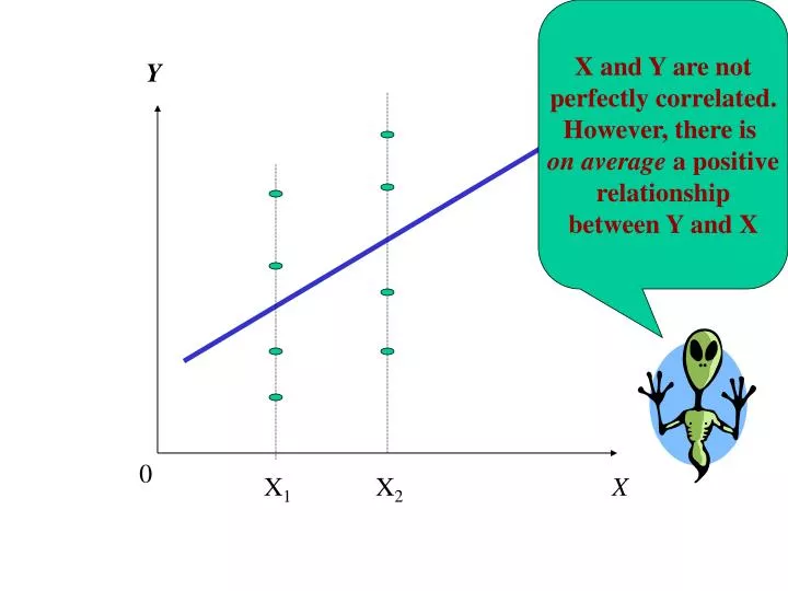
X and Y are not perfectly correlated. However, there is on average a positive relationship between Y and X. Y. 0. X 1. X 2. X. We assume that expected conditional values of Y associated with alternative values of X fall on a line. Y. E(Y i /X i ) = 0 + 1 X i. Y 1. 1.

E N D
X and Y are notperfectly correlated.However, there is on average a positive relationshipbetween Y and X Y 0 X1 X2 X
We assume that expectedconditional values of Yassociated with alternativevalues of X fall on a line. Y E(Yi/Xi) = 0 + 1Xi Y1 1 1 = Y1 - E(Y1/X1) E(Y1/X1) 0 X1 X
The 4 steps of Forecasting • Specification • Estimation • Evaluation • Forecasting
1. Specification Econometric models posit causal relationships among economic variables.Simple regression analysis is used totest the hypothesis about the relationshipbetween a dependent variable (Y, or in our case, C)and independent variable (X, or in our case, Y)). Our model is specified as follows:C = f (Y), whereC: personal consumption expenditureY: Personal disposable income
2. Estimation Simple linear regression begins by plotting C-Y values (see table 1)on a scatter diagram (see figure 1) to determine if there exists an approximate linear relationship: Since the datapoints are unlikely to fallexactly on a line, (1)must be modifiedto include a disturbanceterm (ui) (1) (2) • 0 and 1 are called parameters or population parameters. • We estimate these parameters using the data we have available
We estimate the values of 0 and 1 using the Ordinary Least Squares (OLS) method. OLS is a technique for fitting the "best" straight line to the sample of XY observations. The line of best fit is that which minimizes the sum of the squared (vertical) deviations of the sample points from the line: • Where,Ci are the actual observations of consumption are fitted values of consumption
C The residual C1 e1 0 Y1 Y
The OLS estimators--single variable case are estimators of the true parameters 0 and 1 Note that we use X to denote the explanatoryvariable and Y is the dependent variable.
Thus, we have: Thus the equation obtained from the regression is:
3. Evaluation These statistics tell us how well the equation obtained from the regression performsin terms of producing accurate forecasts • Goodness of fit criteria • Standard errors of the estimates • Are the estimates statistically significant? • Constructing confidence intervals • The coefficient of determination (R2). • The standard error of the regression
Standard errors of the estimates We assume that the regression coefficients are normally distributed variables. The standard error (or standard deviation) of the estimates is a measure of the dispersion of the estimates around their mean value. As a general principle, the smaller the standard error, the better the estimates (in terms of yielding accurate forecasts of the dependent variable). The following rule-of-thumb is useful:"[the] standard error of the regression coefficient should be less than half of the size of [the] corresponding regression coefficient." Let denote the standard error of our estimate of the slope parameter
Note that: By reference to the SPSS output, we see that the standard error of our estimateof 1 is 0.049, whereas our estimate of 1 is 0.861. Hence our estimate is about 17 times the size of its standard error
The t-test • To test for the significance of our estimate of 1, we set the following null hypothesis, H0, and the alternative hypothesis, H1 • H0: 1 0 • H1: 1 > 0 • The t distribution is used to test for statistical significance of the estimate: The t test is a wayof comparing the errorsuggested by the nullhypothesis to the standard error of the estimate A rule-of thumb: if t > 2, reject H0
Constructing confidence intervals To find the 95 percent confidence interval for 1, that is: Pr( a < 1 < b) = .95 To find the upper and lower boundaries of the confidence interval (a and b): Where tc is the critical value of t at the 5 percent confidence level (two-sided,10 degrees of freedom ). tc = 2.228. Working it out, we have: Pr( .752< 1 < .970) = .95 • We can be 95 percent confident that the true value of the slope coefficient is in this range.
The coefficient of determination (R2) • The coefficient of determination, R2, is defined as the proportion of the total variation in the dependent variable (Y) "explained" by the regression of Y on the independent variable (X). The total variation in Y or the total sum of squares (TSS) is defined as: Note: The explained variation in the dependent variable(Y) is called the regression sum of squares (RSS) and is given by:
What remains is the unexplained variation in the dependent variable or theerror sum of squares (ESS) • We can say the following: • TSS = RSS + ESS, or • Total variation = Explained variation + Unexplained variation R2 is defined as:
Note that: 0 R2 1 • If R2 = 0, all the sample points lie on a horizontal line or in a circle • If R2 = 1, the sample points all lie on the regression line • In our case, R2 0.984, meaning that 98.4 percent of the variation in the dependent variable (consumption) is explained by the regression. Think of R2 as the proportion of the total deviation of the dependent variable from its mean value that is accounted for by the explanatory variable(s).
Standard error of the regression • The standard error of the regression (s)is given by • In our case, s = 3.40 • Regression is based on the assumption that the error term is normally distributed, so that 6.87% of the actual values of the dependent variable should be within one standard error ($3.4 billion in our example) of their fitted value. • Also, 95.45% of the observed values of consumption should be within 2 standard errors of their fitted values ($6.8 billion).
IV. Forecasting Our forecasting equation was estimated as follows: • At the most basic level, forecasting consists of inserting forecasted values of the explanatory variable X (disposable income) into the forecasting equation to obtain forecasted values of the dependent variable Y (personal consumption expenditure).
Can we make a good forecast? • Our ability to generate accurate forecasts of the dependent variable depends on two factors: • Do we have good forecasts of the explanatory variable? • Does our model exhibit structural stability, i.e., will the causal relationship between C and Y expressed in our forecasting equation hold up over time? After all, the estimated coefficients are average values for a specific time interval (1987-1998). While the past may be a serviceable guide to the future in the case of purely physical phenomena, the same principle does not necessarily hold in the realm of social phenomena (to which economy belongs).
Having forecastedvalues of income in hand, we can forecastconsumption through the year 2003