Download
1 / 20
200 likes | 318 Vues
Anna Atramentov Dept. of Computer Science Iowa State University Ames, IA, USA. Steven M. LaValle Dept. of Computer Science University of Illinois Urbana, IL, USA. Efficient Nearest Neighbor Searching for Motion Planning. Support provided in part by an NSF CAREER award. Statistics

E N D
Anna Atramentov Dept. of Computer Science Iowa State University Ames, IA, USA Steven M. LaValle Dept. of Computer Science University of Illinois Urbana, IL, USA Efficient Nearest Neighbor Searching for Motion Planning Support provided in part by an NSF CAREER award.
Statistics Pattern recognition Machine Learning Motivation In motion planning the following algorithms rely heavily on nearest neighbor algorithms: • PRM-based methods • RRT-based methods Nearest neighbor searching is a fundamental problem in many applications:
Given: 2D or 3D world Geometric models of a robot and obstacles Configuration space Initial and goal configurations Task: Compute a collision free path that connects initial and goal configurations Basic Motion Planning Problem
Probabilistic roadmap approaches(Kavraki, Svestka, Latombe, Overmars, 1994) The precomputation phase consists of the following steps: • Generate vertices in configuration space at random • Connect close vertices • Return resulting graph • The query phase: • Connect initial and goal to graph • Search the graph Obstacle-Based PRM (Amato, Wu, 1996); Sensor-based PRM (Yu, Gupta, 1998); Gaussian PRM (Boor, Overmars, van der Stappen, 1999); Medial axis PRMs (Wilmarth, Amato, Stiller, 1999; Psiula, Hoff, Lin, Manocha, 2000; Kavraki, Guibas, 2000); Contact space PRM (Ji, Xiao, 2000); Closed-chain PRMs (LaValle, Yakey, Kavraki, 1999; Han, Amato 2000); Lazy PRM (Bohlin, Kavraki, 2000); PRM for changing environments (Leven, Hutchinson, 2000); Visibility PRM (Simeon, Laumond, Nissoux, 2000).
xinit Rapidly-exploring random tree approaches GENERATE_RRT(xinit, K, t) • T.init(xinit); • For k = 1 to K do • xrand RANDOM_STATE(); • xnear NEAREST_NEIGHBOR(xrand, T); • u SELECT_INTPUT(xrand, xnear); • xnew NEW_STATE(xnear, u, t); • T.add_vertex(xnew); • T.add_edge(xnear, xnew, u); • Return T; xrand xnew xnear The result is a tree rooted at xinit: LaValle, 1998; LaValle, Kuffner, 1999, 2000; Frazzoli, Dahleh, Feron, 2000; Toussaint, Basar, Bullo, 2000; Vallejo, Jones, Amato, 2000; Strady, Laumond, 2000; Mayeux, Simeon, 2000; Karatas, Bullo, 2001; Li, Chang, 2001; Kuffner, Nishiwaki, Kagami, Inaba, Inoue, 2000, 2001; Williams, Kim, Hofbaur, How, Kennell, Loy, Ragno, Stedl, Walcott, 2001; Carpin, Pagello, 2002.
Goals • ANN (U. of Maryland) • Ranger (SUNY Stony Brook) Existing nearest neighbor packages: Problem: They only work for Rn. Configuration spaces that usually arise in motion planning are products of R, S1 and projective spaces. Theoretical results: P. Indyk, R. Motwani, 1998; P. Indyk, 1998, 1999; Problem: Difficulty of implementation Our goal: Design simple and efficient algorithm for finding nearest neighbor in these topological spaces
Literature on NN searching • It is very well studied problem • Kd-tree approach is very simple and efficient • T. Cover, P. Hart, 1967 • D. Dobkin, R. Lipton, 1976 • J. Bentley, M. Shamos, 1976 • S. Arya, D. Mount, 1993, 1994 • M. Bern, 1993 • T. Chan, 1997 • J. Kleinberg, 1997 • K. Clarkson, 1988, 1994, 1997 • P. Agarwal, J. Erickson, 1998 • P. Indyk, R. Motwani, 1998 • E. Kushilevitz, R. Ostrovsky, Y. Rabani, 1998 • P. Indyk, 1998, 1999 • A. Borodin, R. Ostrovsky, Y. Rabani, 1999
Problem Formulation Given a d-dimensional manifold, T, represented as a polygonal schema, and a set of data points in T. Preprocess these points so that, for any query point qT, the nearest data point to q can be found quickly. The manifolds of interest: • Euclidean one-space, represented by (0,1) R. • Circle, represented by [0,1], in which 0 1 by identification. • P3, represented by [0, 1]3 with antipodal points identified. Examples of 4-sided polygonal schemas: cylinder torus projective plane
4 4 4 4 4 4 4 4 6 6 6 6 6 6 6 6 7 7 7 7 7 7 7 7 8 8 8 8 8 8 8 8 5 5 5 5 5 5 5 5 9 9 9 9 9 9 9 9 10 10 10 10 10 10 10 10 3 3 3 3 3 3 3 3 2 2 2 2 2 2 2 2 1 1 1 1 1 1 1 1 11 11 11 11 11 11 11 11 Example: a torus 4 6 7 q 8 5 9 10 3 2 1 11
Algorithm presentation • Overview of the kd-tree algorithm • Modification of kd-tree algorithm to handle topology • Analysis of the algorithm • Experimental results
4 6 l1 l9 7 l5 l6 8 l3 l2 5 9 10 3 l10 l8 l7 2 5 4 11 8 2 1 l4 11 1 3 9 10 6 7 Kd-trees The kd-tree is a powerful data structure that is based on recursively subdividing a set of points with alternating axis-aligned hyperplanes. The classical kd-tree uses O(dnlgn) precomputation time, O(dn) space and answers queries in time logarithmic in n, but exponential in d. l1 l3 l2 l4 l5 l7 l6 l8 l10 l9
4 6 l1 7 8 5 9 10 3 2 1 11 2 5 4 11 8 1 3 9 10 6 7 Kd-trees. Construction l9 l1 l5 l6 l3 l2 l3 l2 l10 l4 l5 l7 l6 l8 l7 l4 l8 l10 l9
l1 q 2 5 4 11 8 1 3 9 10 6 7 Kd-trees. Query 4 6 l9 l1 7 l5 l6 l3 8 l2 l3 l2 5 9 10 3 l10 l4 l5 l7 l6 l8 l7 2 1 l4 11 l8 l10 l9
l1 l3 l2 l4 l5 l7 l6 l8 l10 l9 l1 l2 4 6 l9 7 l5 3 l6 l8 8 l3 l2 5 1 l4 9 10 3 l10 l8 l7 2 1 l4 11 q 2 5 4 11 8 1 3 9 10 6 7 Algorithm Presentation
Analysis of the Algorithm Proposition 1. The algorithm correctly returns the nearest neighbor. Proof idea:The points of kd-tree not visited by an algorithm will always be further from the query point then some point already visited. Proposition 2. For n points in dimension d, the construction time is O(dnlgn), the space is O(dn), and the query time is logarithmic in n, but exponential in d. Proof idea:This follows directly from the well-known complexity of the basic kd-tree.
Experiments For 50,000 data points 100 queries were made:
Conclusion • We extended kd-tree to handle topology of the configuration space • We have presented simple and efficient algorithm • We have developed software for this algorithm which will be included in Motion Strategy Library (http://msl.cs.uiuc.edu/msl/) Future Work • Extension to more efficient kd-trees • Extension to different topological spaces • Extension to different metric spaces