Download
1 / 59
620 likes | 925 Vues
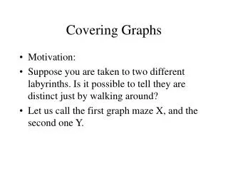
Covering Graphs. Motivation: Suppose you are taken to two different labyrinths. Is it possible to tell they are distinct just by walking around? Let us call the first graph maze X, and the second one Y. Question. Is it possible to distinguish between the two mazes?

E N D
Covering Graphs • Motivation: • Suppose you are taken to two different labyrinths. Is it possible to tell they are distinct just by walking around? • Let us call the first graph maze X, and the second one Y.
Question • Is it possible to distinguish between the two mazes? • Answer: Yes, we can. In the upper maze there are two adjacent trivalent vertices. This is not the case in the lower maze.
Local Isomorphism • On the other hand we cannot distinguish (locally) between the upper and lower graph. • To each walk upstairs we can associate a walk downstairs.
One More Example • C4 over C3 is no good. However, C6 over C3 is Ok.
Fibers and Sheets. • We say that C6 is a twosheeted cover over C3. Red vertices are in the same fiber. Similarly, the dotted lines belong to the saem fiber. • Graph mapping f: C6 C3 is called covering projection. • Preimage of a vertex f-1(v) (or an edge f-1(e)) is called a fiber. • The cardinality of a fiber is constant. k =|f-1(v)| is called the number of sheets.
One More Example • The cube graph Q3 is a two fold cover over complete graph K4. • The vertex fibers are composed of pairs of antipodal vertices.
Covers over Pregraphs • Graph K4 can be understood as a four-fold cover over a pregraph on one vertex (one loop and one half-edge).
Voltage Graphs • X = (V,S,i,r) – connected (pre)graph. • (G,A) – permutation group acting on space A. • g:S G – voltage assignment. • Condition: for each s 2 S we have g[s]g[r(s)] = id.
Voltage Graph Determines a Covering Graph • Each voltage graph (X,G,A,g) determines a covering graph Y and the covering projection f: Y X as follows: • Covering graph Y = (V(Y),S(Y),i,r) • V(Y) := V(X) x A • S(Y) := S(X) x A • i: S(Y) V(Y): i(s,a) := (i(s),a). • r: S(Y) S(Y): r(s,a) := (r(s), g[s](a)). • Covering projection f • f: V(Y) V(X): f(x,a) := x. • f: S(Y) S(X): f(s,a) := s. • Sometimes we denote the covering graph Y by Cov(X;).
(Rhetorical) Questions • “Different” voltage graphs may give rise to the “same” cover. What does it mean the “same” and how do we obtain all “different” voltage graphs? • The voltage graph is determined in essence by the abstract group. What is the role of permutation group? • How do we ensure that if X is connected then Y is connected, too?
Kronecker Cover • Let X be a graph. The canonical double cover or Kronecker cover: KC(X) is a twofold cover that is defined by a voltage graph that has nontrivial voltage from Z2 on each of its edges. It can also be described as the tensor product KC(X) = X £ K2.
Homework • H1: Prove that Kronecker cover is bipartite. • H2: Prove that generalized Petersen graph G(10,2) is a twofold cover over the Petersen graph G(5,2). • H3: Determine the Kronecker cover over G(5,2). • H4: Determine a Zn covering over the handcuff graph G(1,1), that is not a generalized Petersen graph G(n,r).
Regular Covers • Let Y be a cover over X. We are interested in fiber preserving elements of Aut Y (covering transformations). • Let Aut(Y,X) · Aut Y be the group of covering transformations. • The cover Y is regular, if Aut(Y,X) acts transitively on each fiber. • Regular covers are denoted by voltage graphs, where permutation group (G, A) acts regularly on itself by left or right translations: (G, G).
Exercises • N1: Prove that each double sheeted cover is regular. • N2: Find an example of a three sheeted cover that is not regular. • N3: Express the graph on the left as a 6-fold cover over a pregraph on a single vertex.
Dipole qn • Dipole qn has two vertices joined by n parallel edges. We may call one vertex black, the other white. On the left we see q5. • Each dipole is bipartite, that is why each cover over n is bipartite too. Dipole q3 jeis cubic, sometimes called the theta graphq.
Cyclic cover over a dipole – Haar graph H(n). • H(37) is determined by number 37, actually by its binary representation (1 0 0 1 0 1). • k = 6 is the length of the sequence, hence group Z6. • (0 1 2 3 4 5) – positions of “1”. • Positions of “1”s: 0, 3 in 5. {0,3,5} are the voltages on . The corresponding covering graph is H(37). 0 3 5 Z6
Exercises • Graph on the left is called the Heawood graph H. Prove: • H is bipartite. • H is a Haar graph (Determine n, such that H = H(n)) • Express H as a cyclic cover over . • Show that there are no cycles of lenght < 6 in H. • Show that H is the smallest cubic graph with no cycles of length < 6.
Cages as Covering Graphs • A g-cage is a cubic graph of girth g that has the least number of vertices. • Small cages can be readily described as covering graphs.
1-Cage • Usually we consider only simple graphs. For our purposes it makes sense to define also a 1-cage as a pregraph on the left. • 1-cage is the unique smallest cubic pregraph.
2-Cage • The only 2-cage is the graph. • We may view 2-cage, as the Kronecker cover over 1-cage. 1 1 Z2
K4, the 3-cage 3 2 • K4 is a Z4 covering over the 1-cage. • In general, we obtain a Z2n covering over the 1-cage by assigning voltage 1 to the loop and voltage n to the half-edge. • Exercise: What is the covering graph in such a case? 1 0 2 1 Z4
K3,3, the 4-cage 5 4 • K3,3 is a Z6 covering over the 1-cage. • It can also be seen as a Z3 covering over the 2-cage . • Exercise: Express K3,3 as a covering graph over . Dtermine a natural number n, such that K3,3 is a Haar graph H(n). 3 2 1 0 3 1 Z6
The Handcuff Graph G(1,1) • By changing the voltage on the loop of the 1-cage we obtain a double cover G(1,1), the smallest generalized Petersen graph, known as the Handcuff graph. 1 0 Z2
0 i Zn j I graphs I(n,i,j) and Generalized Petersen graphs G(n,k) • Cyclic covers over the handcuff graph are called I-graphs. Each I-graph can be described by three parameters I(n,i,j) with i · j. In case i = 1 we call I(n,i,k) = G(n,k), the generalized Petersen graph. • In particular, I(5,1,2) is the 5-cage.
b a D7 The 6-cage • The 6-cage is the Heawood graph on 14 vertices. It is a 7-fold cyclic cover over the graph. But it is also a dihedral cover over the 1-cage. • Let the presentaion of Dn be given as follows: Dn = <a,b|an,b2, ab=ba-1> • Then the Heawood is a covering described on the left.
Exercises • N1. Express the 7-cage as a covering graph. • N2. Express the 8-cage as a covering graph.
(3,1)-trees • A (3,1)-tree is a tree whose vertices have valence 3 and 1 only. • On the left we see the smallest (3,1)-trees I,Y and H.
(3,1)-cubic graphs • A (3,1)-cubic graph is obtained from a (3,1)-tree by adding a loop at each vertex of valence 1. • On the left we see the smallest (3,1)-cubic graphs I(1,1,1),Y(1,1,1,1) and H(1,1,1,1,1).
Coverings over (3,1)-cubic graphs Zn j i • By putting 0 on the tree edges and appropriate voltages on the loops of (3,1)-cubic graph we obtain their Zn coverings. • In the case of the graphs on the left we obtain the I-graphs, Y-graphs and H-graphs: I(n,i,j),Y(n,i,j,k) and H(n,i,j,k,l). j i k k i j l
Covers Determined by Graphs • We know already that there exists a cover, namely Kronecker cover, that depends only on X itself and the voltage assignment plays a minor role. • Now we will present some covers that have a similar property.
Coverings and Trees • Let X be a connected graph and let Cov(X) denote all connected covers over X: • Cov(X) = {(Y,)| Y connected and : Y ! X, covering projection}. For each connected X we have (X,id) 2 Cov(X). • Proposition: For a connected X we have Cov(X) = {(X,id)} if and only if X is a tree. • This fact holds both for finite and locally finite trees.
Universal cover • Let X, Y and Z be connected graphs and let : Y ! X and :Z ! Y be covering projections. • On the other hand, we may consider the class Cov(X) of all coverings over X. We may introduce a partial order in Cov(X). (Y,) < (Z,) if there exists a covering projection (Z,) 2 Cov(Y) so that = . • Proposition: Any connected finite or locally finite graph X can be covered by some tree T; : T ! X. • Proposition: Any connected finite or locally finite graph X can be covered by at most one tree T. • Proposition: Let : T ! X be a covering projection form a tree to a connected graph X. Then for each covering : Y ! X there exists a covering : T ! Y such that = . • Corollary: For each connected X the poset Cov(X) has a maximal element (T,) where T is a tree. • The maximal element (T,) 2 Cov(X) is called the universal covering of X.
Construction of Universal Cover • There is a simple construction of the universal covering projection. • Let X be a connected graph and let T µ X be a spanning tree. Furthermore, let S = E(G) \ E(T) be the set of edges not in tree T. • Consider S to be the set of generators for a free group F(S) and F(S) to be the voltage group. • Let us assing voltages on E(G) as follows: • If e 2 E(T) the voltage on e is identity. • If e 2 S the voltage is the corresponding generator (or its inverse) • Note: The construction does not depend on the choice of direction of edges. • Proposition: The described construction gives rise to the universal cover.
Examples • Example: The universal cover over any regular k-valent graph is a regular infinte tree T(1,k).
Valence Partition and Valence Refinement • Let G be a graph and let B = {B1, ..., Bk} be a partition of its vertex set V(G) for which there are constants rij, 1 · i,j · k such that for each v 2 Bi there are rij edges linking v to the vertices in Bj. Let R = [rij] be the corresponding k £ k matrix, Then B is called valence partition and R is called valence refinement. If k is minimal, then B is called minimalvalence partition and R is called minimal valence refinement. • Two refinements R and R’ are considered the same if one can be transformed to the other one by simultaneous permutation of rows and columns. • A refinement is uniform, if each row is constant.
Construction • Given graphs G and G’ with a common refinement. • Let mij denote the number of arcs in G of type i ! j. • Let ni denote the number of vertices in G of type i. • Let bij = lcm(mij)/mij. (If mij = 0 , let bij undefined). • Let ai = lcm(mij)/ni. • Note that bij and ai depend only on the common matrix R and are the same for both graphs G and G’. • Let l(e) or l(e’) be a linear order given to all type i ! j arcs with a common initial vertex i(e) (or i(e’)). • Let V(H) = {(i,v,v’,p)|v and v’ of type i, p 2Zai} • Let S(H) = {(i,j,e,e’,q)|e and e’ of type i ! j, q 2Zbij} • r(i,j,e,e’,q) := (j,i,r(e),r(e’),q) • i(i,j,e,e’,q) := (i,i(e),i(e’),q rij + l(e)-l(e’)} • H is a common cover of G and G’.
Computing Minimal Valence Refinement • Let r[u,B] denote the number of edges linking u to the vertices in B. • Algorithm [F.T.Leighton, Finite Common Coverings of Graphs, JCT(B) 33 1982, 231-238.] • Step 1. Place two vertices in the same block if and only if they have the same valence. • Step 2. While there exist two blocks B and B’ and two distinct vertices u,v in B with r[u,B’] r[v,B’] repeat the following: • Partition the block B into subblocks in such a way that two vertices u,b of B remain in the same block if and only if r[u,B’] = r[v,B’] for each B’ of the previous partition. • Step 3. From minimal valence partition B compute the minimal vertex refinement R. • Note: We may maintain R during the run of the algorithm as a matrix whose elements are sets of numbers.
Comon Cover • Theorem. Given any two finite graphs G and H, the following statements are equivalent: • G and H have the same universal cover, • G and H have a common finite cover, • G and H have a common cover, • G and H have the same minimal valence refinement. • G and H have the same some valence refinement. • Homework. Find the result in the literature and construct a finite comon cover of G(5,2) and G(6,2).
Petersen graph • An unusual drawing of Petersen graph.
Kronecker Cover - Revisited • Kronecker cover KC(G) is an example of covers, determined by the graph itself. • Exercise. Show that G(5,2) and X have the same Kronecker cover.
THE covering graph • Let G be a graph with the vertex set V. By THE(G) we denote the following covering graph. • To each edge e = uv we assing transposition e = (u,v) 2 Sym(V). The resulting covering graph has two components, one being isomorphic to G. The other componet is called THE covering graph.
Examples • On the left we see The covering graph of K2,2,2. • The construction resembles truncation. • Each vertex is truncated and an inverse figure is placed in the space provided for it. • Theorem: If G is planar, then THE(G) is planar.
Homework • H1. Given connected graph G with n vertices and e edges and with valence sequence (d1, d2, ..., dn). Determine the parameters for THE(G). • H2. Determine all connected graphs G for which girth(G) girth(THE(G)).
The fundamental group of a graph. • Let G be a connected graph rooted at r 2 V(G) and let denote the collection of closed walks rooted at r. • Let and be two closed walks rooted at r. The compositum is also a closed walk rooted at r. • We may also define -1 as the inverse walk. • Finally, we need equality (equivalence). • 12 ~ 1 e e-12. • (G,r) := /~ is a group, called the fundamental group of G (first homotopy group). • Fact: (G,r) is a free group generated with m-n+1 generators.
The first Homology group of a graph • Let G be a connected graph and T one of its spanning trees. Each edge h 2 G\T of the co-tree defines a unique cycle C(h) µ E(G). • The charactersitic vector h2 {0,1}m, h(e) = 1, if e 2 C(h) and h(e) = 0, represents C(h). The set of all charactersitic vectors spans a m-n+1 dimensional Z-module in Zm. This can be also viewed as a free abelian group isomorphic to Zm-n+1. • This group is called the first homology group H1(G,Z). We may replace Z by Zk and obtain the first Zk homology groupZkm-n+1.
Pseudohomological Covers • Idea: Let G be a graph and T its spanning tree and with the edges H = {h1,h2,...,hm-n+1} = E(G)\E(T). Let (H) be a group with m-n+1 interchangeable generators H. The pseudohomological-cover HOM(G,,T) is determined by a voltage graph with (e) = id, for e 2 E(T) and (h) = h, for h 2 E(G)\E(T). • Main Question. Is HOM(G,,T) independent of the choice of T and the selection of the generators or their inverses? If the answer is yes, the covering is called homological cover.
Pseudohomological 2-cover • Let G be a graph and T its spanning tree.The pseudohomological 2-cover HOM(G,Z2,T) is determined by a voltage graph with (e) = 0, for e 2 E(T) and (e) = 1, for e E(T). • Theorem. If G is connected then HOM(G,Z2,T) is connected if and only if G is not a tree.
Example 0 • The two voltage graphs on the left determine different pseudohomological Z2 covers. • Cov(G,2) is bipartite and Cov(G,1) is not. 1 0 0 1 1 Z2 0 0 1 1 2 0
Switching • Let (G,) be a voltage graph. Let : V(G) ! be an arbitrary mapping, called switching, that assigns voltages to vertices. Define a new voltage assignment as follows: • (s) := (i(s)) (s) (i(r(s))-1. • is well-defined. • Namely (r(s)) = (i(r(s))) (r(s)) (i(s))-1. • Hence (r(s))-1 = (i(s)) (r(s))-1(i(r(s)))-1 = (i(s)) (s) (i(r(s)))-1 = (s). • Clearly for any switching the graphs Cov(G,) and Cov(G,) coincide. • Given (G,) and any spanning tree T. There exists a switching such that the resulting e is identity on T. • If, in addition, T is rooted at v, we may select (v) = id (or arbitrarily) and this determines switching completely.