Download

1 / 95
950 likes | 1.1k Vues
EECC551 Exam Review. 4 questions out of 6 questions (Must answer first 2 questions and 2 from remaining 4) Instruction Dependencies and graphs In-order Floating Point/Multicycle Pipelining (quiz 2) Improving Instruction-Level Parallelism (ILP). Loop-unrolling (quiz 3)

E N D
EECC551 Exam Review 4 questions out of 6 questions (Must answer first 2 questions and 2 from remaining 4) • Instruction Dependencies and graphs • In-order Floating Point/Multicycle Pipelining (quiz 2) • Improving Instruction-Level Parallelism (ILP). • Loop-unrolling (quiz 3) • Dynamic Pipeline Scheduling. • The Tomasulo Algorithm (quiz 4) • Multiple Instruction Issue (CPI < 1):Superscalar vs. VLIW • Dynamic Hardware-Based Speculation (quiz 5) • Loop-Level Parallelism (LLP). • Making loop iterations parallel (quiz 6) • Software Pipelining (Symbolic Loop-Unrolling) • Cache & Memory Performance. (quiz 7) • I/O & System Performance. (quiz 8)
I .. .. J J (Read) I (Write) J (Read) I (Read) J(Write) J (Write) I (Read) I (Write) Shared Operand Shared Operand Shared Operand Shared Operand Read after Write (RAW) if data dependence is violated Program Order A name dependence: output dependence Write after Write (WAW) if output dependence is violated Data Hazard/Dependence Classification True Data Dependence A name dependence: antidependence Write after Read (WAR) if antidependence is violated No dependence Read after Read (RAR) not a hazard
1 2 3 4 5 6 L.D F0, 0 (R1) ADD.D F4, F0, F2 S.D F4, 0(R1) L.D F0, -8(R1) ADD.D F4, F0, F2 S.D F4, -8(R1) 1 2 3 6 5 4 S.D F4, -8 (R1) L.D F0, -8 (R1) S.D F4, 0(R1) L.D F0, 0 (R1) ADD.D F4, F0, F2 ADD.D F4, F0, F2 Instruction Dependence Example Dependency Graph Example Code Date Dependence: (1, 2) (2, 3) (4, 5) (5, 6) Output Dependence: (1, 4) (2, 5) Anti-dependence: (2, 4) (3, 5) Can instruction 4 (second L.D) be moved just after instruction 1 (first L.D)? If not what dependencies are violated? Can instruction 3 (first S.D) be moved just after instruction 4 (second L.D)? How about moving 3 after 5 (the second ADD.D)? If not what dependencies are violated? What happens if we rename F0 to F6 and F4 to F8 in instructions 4, 5, 6?
if p1 { S1; }; If p2 { S2; } S1 is control dependent on p1 S2 is control dependent on p2 but not on p1 Control Dependencies • Control dependence determines the ordering of an instruction with respect to a branch (control) instruction. • Every instruction in a program except those in the very first basic block of the program is control dependent on some set of branches. • An instruction which is control dependent on a branch cannot be moved before the branch so that its execution is no longer controlled by the branch. • An instruction which is not control dependent on the branch cannot be moved so that its execution is controlled by the branch (in the then portion). • Both scenarios lead a control dependence violation (control hazard). • It’s possible in some cases to violate these constraints and still have correct execution. • Example of control dependence in the then part of an if statement: What happens if S1 is moved here? Control Dependence Violation = Control Hazard In Fourth Edition Chapter 2.1 (In Third Edition Chapter 3.1)
Floating Point/Multicycle Pipelining in MIPS • Completion of MIPS EX stage floating point arithmetic operations in one or two cycles is impractical since it requires: • A much longer CPU clock cycle, and/or • An enormous amount of logic. • Instead, the floating-point pipeline will allow for a longer latency (more EX cycles than 1). • Floating-point operations have the same pipeline stages as the integer instructions with the following differences: • The EX cycle may be repeated as many times as needed (more than 1 cycle). • There may be multiple floating-point functional units. • A stall will occur if the instruction to be issued either causes a structural hazard for the functional unit or cause a data hazard. • The latency of functional units is defined as the number of intervening cycles between an instruction producing the result and the instruction that uses the result (usually equals stall cycles with forwarding used). • The initiation or repeat interval is the number of cycles that must elapse between issuing an instruction of a given type. Solution: to the same functional unit (In Appendix A)
Super-pipelined CPU: A pipelined CPU with pipelined FP units Extending The MIPS Pipeline: Multiple Outstanding Floating Point Operations Latency = 0 Initiation Interval = 1 Latency = 6 Initiation Interval = 1 Pipelined Integer Unit Hazards: RAW, WAW possible WAR Not Possible Structural: Possible Control: Possible Floating Point (FP)/Integer Multiply EX IF ID WB MEM FP Adder Latency = 3 Initiation Interval = 1 Pipelined FP/Integer Divider Latency = 24 Initiation Interval = 25 Non-pipelined In-Order = Start of instruction execution done in program order In-Order Single-Issue MIPS Pipeline with FP Support Pipelined CPU with pipelined FP units = Super-pipelined CPU (In Appendix A)
CC 10 CC 1 CC 2 CC 3 CC 4 CC 5 CC 6 CC 7 CC 8 CC 9 CC 11 CC12 CC13 CC14 CC15 CC16 CC17 CC18 Program Order IF ID M1 M2 M3 M4 M5 M6 M7 WB MEM IF ID A1 A2 A3 A4 WB MEM IF ID EX WB MEM IF ID EX WB MEM STALL STALL STALL STALL STALL STALL STALL STALL STALL STALL STALL STALL STALL STALL STALL STALL STALL FP Code RAW Hazard Stalls Example(with full data forwarding in place) FP Multiply Functional Unit has 7 EX cycles (and 6 cycle latency 6 = 7-1) FP Add Functional Unit has 4 EX cycles (and 3 cycle latency 3 = 4-1) L.D F4, 0(R2) MUL.D F0, F4, F6 ADD.D F2, F0, F8 S.D F2, 0(R2) When run on In-Order Single-Issue MIPS Pipeline with FP Support With FP latencies/initiation intervals given above Third stall due to structural hazard in MEM stage 6 stall cycles which equals latency of FP multiply functional unit (quiz 2) (In Appendix A)
Increasing Instruction-Level Parallelism (ILP) i.e independent or parallel loop iterations • A common way to increase parallelism among instructions is to exploit parallelism among iterations of a loop • (i.e Loop Level Parallelism, LLP). • This is accomplished by unrolling the loop either statically by the compiler, or dynamically by hardware, which increases the size of the basic block present. This resulting larger basic block provides more instructions that can be scheduled or re-ordered by the compiler to eliminate more stall cycles. • In this loop every iteration can overlap with any other iteration. Overlap within each iteration is minimal. for (i=1; i<=1000; i=i+1;) x[i] = x[i] + y[i]; • In vector machines, utilizing vector instructions is an important alternative to exploit loop-level parallelism, • Vector instructions operate on a number of data items. The above loop would require just four such instructions. Or Data Parallelism in a loop 4 vector instructions: Load Vector X Load Vector Y Add Vector X, X, Y Store Vector X Independent (parallel) loop iterations: A result of high degree of data parallelism (potentially) In Fourth Edition Chapter 2.2 (In Third Edition Chapter 4.1)
R1 initially points here High Memory X[1000] First element to compute R1 -8 points here X[999] . . . . Program Order R2 +8 points here Last element to compute X[1] R2 points here Low Memory MIPS Loop Unrolling Example • For the loop: for (i=1000; i>0; i=i-1) x[i] = x[i] + s; The straightforward MIPS assembly code is given by: Loop: L.D F0, 0 (R1) ;F0=array element ADD.D F4, F0, F2 ;add scalar in F2 (constant) S.D F4, 0(R1) ;store result DADDUI R1, R1, # -8 ;decrement pointer 8 bytes BNE R1, R2,Loop ;branch R1!=R2 Note: Independent Loop Iterations S R1 is initially the address of the element with highest address. 8(R2) is the address of the last element to operate on. Basic block size = 5 instructions X[ ] array of double-precision floating-point numbers (8-bytes each) In Fourth Edition Chapter 2.2 (In Third Edition Chapter 4.1) • (quiz 3) Initial value of R1 = R2 + 8000
Instruction Producing Result FP ALU Op FP ALU Op Load Double Load Double Instruction Using Result Another FP ALU Op Store Double FP ALU Op Store Double Latency In Clock Cycles 3 2 1 0 MIPS FP Latency For Loop Unrolling Example • All FP units assumed to be pipelined. • The following FP operations latencies are used: (or Number of Stall Cycles) i.e followed immediately by .. i.e 4 execution (EX) cycles for FP instructions Other Assumptions: - Branch resolved in decode stage, Branch penalty = 1 cycle - Full forwarding is used - Single Branch delay Slot - Potential structural hazards ignored In Fourth Edition Chapter 2.2 (In Third Edition Chapter 4.1)
Program Order Loop Unrolling Example (continued) • This loop code is executed on the MIPS pipeline as follows: (Branch resolved in decode stage, Branch penalty = 1 cycle, Full forwarding is used) No scheduling Clock cycle Loop: L.D F0, 0(R1) 1 stall 2 ADD.D F4, F0, F2 3 stall 4 stall 5 S.D F4, 0 (R1) 6 DADDUI R1, R1, # -8 7 stall 8 BNE R1,R2, Loop 9 stall 10 10 cycles per iteration Scheduled with single delayed branch slot: Loop: L.D F0, 0(R1) DADDUI R1, R1, # -8 ADD.D F4, F0, F2 stall BNE R1,R2, Loop S.D F4,8(R1) 6 cycles per iteration (Resulting stalls shown) (Resulting stalls shown) Cycle 1 2 3 4 5 6 Due to resolving branch in ID S.D in branch delay slot 10/6 = 1.7 times faster • Ignoring Pipeline Fill Cycles • No Structural Hazards In Fourth Edition Chapter 2.2 (In Third Edition Chapter 4.1)
4 1 2 3 Three branches and three decrements of R1 are eliminated. Load and store addresses are changed to allow DADDUI instructions to be merged. The unrolled loop runs in 28 cycles assuming each L.D has 1 stall cycle, each ADD.D has 2 stall cycles, the DADDUI 1 stall, the branch 1 stall cycle, or 28/4 = 7 cycles to produce each of the four elements. Loop unrolled 4 times Cycle Loop Unrolling Example (continued) Iteration No scheduling Loop: L.D F0, 0(R1) Stall ADD.D F4, F0, F2 Stall Stall SD F4,0 (R1); drop DADDUI & BNE LD F6, -8(R1) Stall ADDD F8, F6, F2 Stall Stall SD F8, -8 (R1),; drop DADDUI & BNE LD F10, -16(R1) Stall ADDD F12, F10, F2 Stall Stall SD F12, -16 (R1); drop DADDUI & BNE LD F14, -24 (R1) Stall ADDD F16, F14, F2 Stall Stall SD F16, -24(R1) DADDUI R1, R1, # -32 Stall BNE R1, R2, Loop Stall 1 2 3 4 5 6 7 8 9 10 11 12 13 14 15 16 17 18 19 20 21 22 23 24 25 26 27 28 • The resulting loop code when four copies of the loop body are unrolled without reuse of registers. • The size of the basic block increased from 5 instructions in the original loop to 14 instructions. Register Renaming Used i.e 7 cycles for each original iteration (Resulting stalls shown) In Fourth Edition Chapter 2.2 (In Third Edition Chapter 4.1) i.e. unrolled four times Note use of different registers for each iteration (register renaming)
Program Order Larger Basic Block More ILP Loop Unrolling Example (continued) Note: No stalls When scheduled for pipeline Loop: L.D F0, 0(R1) L.D F6,-8 (R1) L.D F10, -16(R1) L.D F14, -24(R1) ADD.D F4, F0, F2 ADD.D F8, F6, F2 ADD.D F12, F10, F2 ADD.D F16, F14, F2 S.D F4, 0(R1) S.D F8, -8(R1) DADDUI R1, R1,# -32 S.D F12, 16(R1),F12 BNE R1,R2, Loop S.D F16, 8(R1), F16 ;8-32 = -24 The execution time of the loop has dropped to 14 cycles, or 14/4 = 3.5 clock cycles per element compared to 7 before scheduling and 6 when scheduled but unrolled. Speedup = 6/3.5 = 1.7 Unrolling the loop exposed more computations that can be scheduled to minimize stalls by increasing the size of the basic block from 5 instructions in the original loop to 14 instructions in the unrolled loop. i.e 3.5 cycles for each original iteration i.e more ILP exposed Exposed In branch delay slot In Fourth Edition Chapter 2.2 (In Third Edition Chapter 4.1)
Dynamic Pipeline Scheduling • Dynamic instruction scheduling is accomplished by: • Dividing the Instruction Decode ID stage into two stages: • Issue: Decode instructions, check for structural hazards. • A record of data dependencies is constructed as instructions are issued • This creates a dynamically-constructed dependency graph for the window of instructions in-flight (being processed) in the CPU. • Read operands: Wait until data hazard conditions, if any, are resolved, then read operands when available (then start execution) (All instructions pass through the issue stage in order but can be stalled or pass each other in the read operands stage). • In the instruction fetch stage IF, fetch an additional instruction every cycle into a latch or several instructions into an instruction queue. • Increase the number of functional units to meet the demands of the additional instructions in their EX stage. • Two approaches to dynamic scheduling: • Dynamic scheduling with the Scoreboard used first in CDC6600(1963) • The Tomasulo approach pioneered by the IBM 360/91(1966) Always done in program order Can be done out of program order (Control Data Corp.) 1 2 CDC660 is the world’s first “Supercomputer” Cost: $7 million in 1963 Fourth Edition: Appendix A.7, Chapter 2.4 (Third Edition: Appendix A.8, Chapter 3.2)
Tomasulo Algorithm Vs. Scoreboard • Control & buffers distributedwith Functional Units (FUs) Vs. centralized in Scoreboard: • FU buffers are called “reservation stations” which have pending instructions and operands and other instruction status info (including data dependencies). • Reservations stations are sometimes referred to as “physical registers” or “renaming registers” as opposed to architecture registers specified by the ISA. • ISA Registers in instructions are replaced by either values (if available) or pointers (renamed) to reservation stations (RS) that will supply the value later: • This process is called register renaming. • Register renaming eliminates WAR, WAW hazards (name dependence). • Allows for a hardware-based version of loop unrolling. • More reservation stations than ISA registers are possible, leading to optimizations that compilers can’t achieve and prevents the number of ISA registers from becoming a bottleneck. • Instruction results go (forwarded) from RSs to RSs , not through registers, over Common Data Bus (CDB)that broadcasts results to all waiting RSs (dependant instructions). • Loads and Stores are treated as FUs with RSs as well. Register Renaming Forwarding In Fourth Edition: Chapter 2.4 (In Third Edition: Chapter 3.2)
Dynamic Scheduling: The Tomasulo Approach (Instruction Fetch) Instructions to Issue (in program order) (IQ) The basic structure of a MIPS floating-point unit using Tomasulo’s algorithm In Fourth Edition: Chapter 2.4 (In Third Edition: Chapter 3.2) Pipelined FP units are used here
Reservation Station (RS) Fields When available • Op Operation to perform in the unit (e.g., + or –) • Vj, VkValue of Source operands S1 and S2 • Store buffers have a single V field indicating result to be stored. • Qj, Qk Reservation stations producing source registers. (value to be written). • No ready flags as in Scoreboard; Qj,Qk=0 => ready. • Store buffers only have Qi for RS producing result. • A: Address information for loads or stores. Initially immediate field of instruction then effective address when calculated. • Busy: Indicates reservation station is busy. • Register result status: Qi Indicates which Reservation Station will write each register, if one exists. • Blank (or 0) when no pending instruction (i.e. RS) exist that will write to that register. RS’s (i.e. operand values needed by instruction) In Fourth Edition: Chapter 2.4 (In Third Edition: Chapter 3.2) Register bank behaves like a reservation station
Three Stages of Tomasulo Algorithm Always done in program order • Issue:Get instruction from pending Instruction Queue (IQ). • Instruction issued to a free reservation station(RS) (no structural hazard). • Selected RS is marked busy. • Control sends available instruction operands values (from ISA registers) to assigned RS. • Operands not available yet are renamed to RSs that will produce the operand (register renaming). (Dynamic construction of data dependency graph) • Execution (EX): Operate on operands. • When both operands are ready then start executing on assigned FU. • If all operands are not ready, watch Common Data Bus (CDB) for needed result (forwarding done via CDB). (i.e. wait on any remaining operands, no RAW) • Write result (WB):Finish execution. • Write result on Common Data Bus (CDB) to all awaiting units (RSs) • Mark reservation station as available. • Normal data bus: data + destination (“go to” bus). • Common Data Bus (CDB): data + source (“come from” bus): • 64 bits for data + 4 bits for Functional Unit source address. • Write data to waiting RS if source matches expected RS (that produces result). • Does the result forwarding via broadcast to waiting RSs. Stage 0 Instruction Fetch (IF): No changes, in-order Also includes waiting for operands + MEM Data dependencies observed i.e broadcast result on CDB (forwarding) Note: No WB for stores Can be done out of program order Including destination register In Fourth Edition: Chapter 2.4 (In Third Edition: Chapter 3.2)
# of RSs EX Cycles Integer 1 1 Floating Point Multiply/divide 2 10/40 Floating Point add 3 2 Real Data Dependence (RAW) Anti-dependence (WAR) Output Dependence (WAW) Tomasulo Approach Example Using the same code used in the scoreboard example to be run on the Tomasulo configuration given earlier: L.D F6, 34(R2) L.D F2, 45(R3) MUL. D F0, F2, F4 SUB.D F8, F6, F2 DIV.D F10, F0, F6 ADD.D F6, F8, F2 Pipelined Functional Units L.D processing takes two cycles: EX, MEM (only one cycle in scoreboard example) In Fourth Edition: Chapter 2.5 (In Third Edition: Chapter 3.3)
Instruction status Execution Write Instruction j k Issue complete Result Busy Address F6 34+ R2 1 3 4 Load1 No F2 45+ R3 2 4 5 Load2 No L.D F0 F2 F4 3 15 16 Load3 No L.D F8 F6 F2 4 7 8 MUL.D Instruction Block done F10 F0 F6 5 56 57 SUB.D F6 F8 F2 6 10 11 DIV.D Reservation Stations S1 S2 RS for j RS for k ADD.D Time Name Busy Op Vj Vk Qj Qk 0 Add1 No 0 Add2 No Add3 No 0 Mult1 No 0 Mult2 No Register result status F0 F2 F4 F6 F8 F10 F12 ... F30 Clock 57 FU M*F4 M(45+R3) (M–M)+M() M()–M() M*F4/M • We have: • In-oder issue, • Out-of-order execution, completion Tomasulo Example: Cycle 57 • (quiz 4)
Tomasulo Loop Example(Hardware-Based Version of Loop-Unrolling) Loop: L.D F0, 0(R1) MUL.D F4,F0,F2 S.D F4, 0(R1) DADDUI R1,R1, # -8 BNE R1,R2, Loop ; branch if R1 ¹ R2 • Assume FP Multiply takes 4 execution clock cycles. • Assume first load takes 8 cycles (possibly due to a cache miss), second load takes 4 cycles (cache hit). • Assume R1 = 80 initially. • Assume DADDUI only takes one cycle (issue) • Assume branch resolved in issue stage (no EX or CDB write) • Assume branch is predicted taken and no branch misprediction. • No branch delay slot is used in this example. • Stores take 4 cycles (ex, mem) and do not write on CDB • We’ll go over the execution to complete first two loop iterations. Note independent loop iterations 3rd …. i.e. Perfect branch prediction. How? Expanded from loop example in Chapter 2.5 (Third Edition Chapter 3.3)
L.D MUL.D S.D L.D MUL.D S.D L.D F0, 0(R1) Issue MUL.D F4,F0,F2 S.D F4, 0(R1) R1, R1, #-8 DADDUI BNE R1,R2,loop (First two Loop iterations done) Loop Example Cycle 20 Instruction status Execution Write Instruction j k iteration Issue complete Result Busy Address 4 54 F0 0 R1 1 1 9 10 Load1 Yes F4 F0 F2 1 2 14 15 Load2 No F4 0 R1 1 3 19 Load3 No Qi F0 0 R1 2 6 10 11 Store1 No 0 F4 F0 F2 2 7 15 16 Store2 No F4 0 R1 2 8 20 Store3 Yes 64 Mult1 Reservation Stations S1 S2 RS for j RS for k Time Name Busy Op Vj Vk Qj Qk Code: 0 Add1 No 0 Add2 No 0 Add3 No M(64) 1 Mult1 Yes MULTD R(F2) 0 Mult2 No Register result status F0 F2 F4 F6 F8 F10 F12 ... F30 Clock R1 20 56 Qi Load1 Mult1 Second S.D done (No write on CDB for stores) Second loop iteration done Issue fourth iteration L.D (to RS Load1)
1 2 3 4 5 6 7 8 9 10 11 12 13 14 15 16 17 18 19 20 21 L.D. I E E E E E E E E W MUL.D I E E E E W S.D. I E E E E DADDUI I BNE I L.D. I E E E E W MUL.D I E E E E W S.D. I E E E E DADDUI I BNE I L.D. I E E E E W MUL.D I E E E E S.D. I DADDUI I BNE I L.D. I E MUL.D I S.D. DADDUI BNE Tomasulo Loop Example Timing Diagram Cycle Iteration 1 2 3 4 3rd L.D write delayed one cycle 3rd MUL.D issue delayed until mul RS is available I = Issue E = Execute W = Write Result on CDB
Multiple Instruction Issue: CPI < 1 • To improve a pipeline’s CPI to be better [less] than one, and to better exploit Instruction Level Parallelism (ILP), a number of instructions have to be issued in the same cycle. • Multiple instruction issue processors are of two types: • Superscalar: A number of instructions (2-8) is issued in the same cycle, scheduled statically by the compiler or -more commonly- dynamically (Tomasulo). • PowerPC, Sun UltraSparc, Alpha, HP 8000, Intel PII, III, 4 ... • VLIW (Very Long Instruction Word): A fixed number of instructions (3-6) are formatted as one long instruction word or packet (statically scheduled by the compiler). • Example: Explicitly Parallel Instruction Computer (EPIC) • Originally a joint HP/Intel effort. • ISA: Intel Architecture-64 (IA-64) 64-bit address: • First CPU: Itanium, Q1 2001. Itanium 2 (2003) • Limitations of the approaches: • Available ILP in the program (both). • Specific hardware implementation difficulties (superscalar). • VLIW optimal compiler design issues. Most common = 4 instructions/cycle called 4-way superscalar processor 1 2 4th Edition: Chapter 2.7 (3rd Edition: Chapter 3.6, 4.3 CPI < 1 or Instructions Per Cycle (IPC) > 1
Unrolled Loop Example for Scalar (single-issue) Pipeline 1 Loop: L.D F0,0(R1) 2 L.D F6,-8(R1) 3 L.D F10,-16(R1) 4 L.D F14,-24(R1) 5 ADD.D F4,F0,F2 6 ADD.D F8,F6,F2 7 ADD.D F12,F10,F2 8 ADD.D F16,F14,F2 9 S.D F4,0(R1) 10 S.D F8,-8(R1) 11 DADDUI R1,R1,#-32 12 S.D F12,16(R1) 13 BNE R1,R2,LOOP 14 S.D F16,8(R1) ; 8-32 = -24 14 clock cycles, or 3.5 per original iteration (result) (unrolled four times) Latency: L.D to ADD.D: 1 Cycle ADD.D to S.D: 2 Cycles Unrolled and scheduled loop from loop unrolling example Recall that loop unrolling exposes more ILP by increasing size of resulting basic block No stalls in code above: CPI = 1 (ignoring initial pipeline fill cycles)
Loop Unrolling in 2-way Superscalar Pipeline: (1 Integer, 1 FP/Cycle) Integer instruction FP instruction Clock cycle Loop: L.D F0,0(R1) 1 L.D F6,-8(R1) 2 L.D F10,-16(R1) ADD.D F4,F0,F2 3 L.D F14,-24(R1) ADD.D F8,F6,F2 4 L.D F18,-32(R1) ADD.D F12,F10,F2 5 S.D F4,0(R1) ADD.D F16,F14,F2 6 S.D F8,-8(R1) ADD.D F20,F18,F2 7 S.D F12,-16(R1) 8 DADDUI R1,R1,#-40 9 S.D F16,-24(R1) 10 BNE R1,R2,LOOP 11 SD -32(R1),F20 12 • Unrolled 5 times to avoid delays and expose more ILP (unrolled one more time) • 12 cycles, or 12/5 = 2.4 cycles per iteration (3.5/2.4= 1.5X faster than scalar) • CPI = 12/ 17 = .7 worse than ideal CPI = .5 because 7 issue slots are wasted Empty or wasted issue slot Recall that loop unrolling exposes more ILP by increasing basic block size Scalar Processor = Single-issue Processor
Loop Unrolling in VLIW Pipeline(2 Memory, 2 FP, 1 Integer / Cycle) 5-issue VLIW Ideal CPI = 0.2 IPC = 5 Memory Memory FP FP Int. op/ Clockreference 1 reference 2 operation 1 op. 2 branch L.D F0,0(R1) L.D F6,-8(R1) 1 L.D F10,-16(R1) L.D F14,-24(R1) 2 L.D F18,-32(R1) L.D F22,-40(R1) ADD.D F4,F0,F2 ADD.D F8,F6,F2 3 L.D F26,-48(R1) ADD.D F12,F10,F2 ADD.D F16,F14,F2 4 ADD.D F20,F18,F2 ADD.D F24,F22,F2 5 S.D F4,0(R1) S.D F8, -8(R1) ADD.D F28,F26,F2 6 S.D F12, -16(R1) S.D F16,-24(R1) DADDUI R1,R1,#-56 7 S.D F20, 24(R1) S.D F24,16(R1) 8 S.D F28, 8(R1)BNE R1,R2,LOOP 9 Unrolled 7 times to avoid delays and expose more ILP 7 results in 9 cycles, or 1.3 cycles per iteration (2.4/1.3 =1.8X faster than 2-issue superscalar, 3.5/1.3 = 2.7X faster than scalar) Average: about 23/9 = 2.55 IPC (instructions per clock cycle) Ideal IPC =5, CPI = .39 Ideal CPI = .2 thus about 50% efficiency, 22 issue slots are wasted Note: Needs more registers in VLIW (15 vs. 6 in Superscalar) Empty or wasted issue slot Scalar Processor = Single-Issue Processor 4th Edition: Chapter 2.7 pages 116-117 (3rd Edition: Chapter 4.3 pages 317-318)
Multiple Instruction Issue with Dynamic Scheduling Example Assumptions: Restricted 2-way superscalar: 1 integer, 1 FP Issue Per Cycle A sufficient number of reservation stations is available. Total two integer units available: One integer unit (for ALU, effective address) One integer unit for branch condition 2 CDBs Execution cycles: Integer: 1 cycle Load: 2 cycles (1 ex + 1 mem) FP add: 3 cycles Any instruction following a branch cannot start execution until after branch condition is evaluated in EX (resolved) Branches are single issued, no delayed branch, perfect branch prediction 1 2 3 4 5 6 7 8 9 3rd Edition:Example on page 221 (not in 4th Edition)
Three Loop Iterations on Restricted 2-way Superscalar Tomasulo FP EX = 3 cycles (Start) BNE Single Issue BNE Single Issue BNE Single Issue Only one CDB is actually needed in this case. 19 cycles to complete three iterations FP ADD has 3 execution cycles Branches single issue For instructions after a branch: Execution starts after branch is resolved
Multiple Instruction Issue with Dynamic Scheduling Example 3rd Edition: Example on page 223 (Not in 4th Edition) Assumptions: The same loop in previous example On restricted 2-way superscalar: 1 integer, 1 FP Issue Per Cycle A sufficient number of reservation stations is available. Total three integer units one for ALU, one for effective address One integer unit for branch condition 2 CDBs Execution cycles: Integer: 1 cycle Load: 2 cycles (1 ex + 1 mem) FP add: 3 cycles Any instruction following a branch cannot start execution until after branch condition is evaluated Branches are single issued, no delayed branch, perfect branch prediction 1 2 One More 3 4 5 6 7 8 Previous example repeated with one more integer ALU (3 total) 9 Example on page 223
(Start) BNE Single Issue BNE Single Issue BNE Single Issue Both CDBs are used here (in cycles 4, 8) FP EX = 3 cycles Same three loop Iterations on Restricted 2-way Superscalar Tomasulo but with Three integer units (one for ALU, one for effective address calculation, one for branch condition) 16 cycles here vs. 19 cycles (with two integer units) 3rd Edition:page 224 (not in 4th Edition For instructions after a branch: Execution starts after branch is resolved
Dynamic Hardware-Based Speculation (Speculative Execution Processors, Speculative Tomasulo) • Combines: • Dynamic hardware-based branch prediction • Dynamic Scheduling: issue multiple instructions in order and execute out of order. (Tomasulo) • Continue to dynamically issue, and execute instructions passed a conditional branch in the dynamically predicted branch direction, before control dependencies are resolved. • This overcomes the ILP limitations of the basic block size. • Creates dynamically speculated instructions at run-time with no ISA/compiler support at all. • If a branch turns out as mispredicted all such dynamically speculated instructions must be prevented from changing the state of the machine (registers, memory). • Addition of commit (retire, completion, or re-ordering) stage and forcing instructions to commit in their order in the code (i.e to write results to registers or memory in program order). • Precise exceptions are possible since instructions must commit in order. 1 2 i.e. before branch is resolved Why? i.e Dynamic speculative execution i.e speculated instructions must be cancelled How? i.e instructions forced to complete (commit) in program order 4th Edition: Chapter 2.6, 2.8 (3rd Edition: Chapter 3.7)
Commit or Retirement (In Order) Hardware-Based Speculation FIFO Usually implemented as a circular buffer Instructions to issue in order: Instruction Queue (IQ) Speculative Execution + Tomasulo’s Algorithm Next to commit = Speculative Tomasulo Store Results Speculative Tomasulo-based Processor 4th Edition: page 107 (3rd Edition: page 228)
Four Steps of Speculative Tomasulo Algorithm 1.Issue— (In-order) Get an instruction from Instruction Queue If a reservation station and a reorder buffer slot are free, issue instruction & send operands & reorder buffer number for destination (this stage is sometimes called “dispatch”) 2. Execution— (out-of-order) Operate on operands (EX) When both operands are ready then execute; if not ready, watch CDB for result; when both operands are in reservation station, execute; checks RAW (sometimes called “issue”) 3. Write result— (out-of-order) Finish execution (WB) Write on Common Data Bus (CDB) to all awaiting FUs & reorder buffer; mark reservation station available. 4. Commit— (In-order) Update registers, memory with reorder buffer result • When an instruction is at head of reorder buffer & the result is present, update register with result (or store to memory) and remove instruction from reorder buffer. • A mispredicted branch at the head of the reorder buffer flushes the reorder buffer (cancels speculated instructions after the branch) • Instructions issue in order, execute (EX), write result (WB) out of order, but must commit in order. Stage 0 Instruction Fetch (IF): No changes, in-order Includes data MEM read No write to registers or memory in WB No WB for stores i.e Reservation Stations 4th Edition: pages 106-108 (3rd Edition: pages 227-229)
Multiple Issue with Speculation Example(2-way superscalar with no restriction on issue instruction type) i.e issue up to 2 instructions and commit up to 2 instructions per cycle Integer code Ex = 1 cycle Assumptions: A sufficient number of reservation stations and reorder (commit) buffer entries are available. Branches still single issue (quiz 5) 4th Edition: pages 119-121 (3rd Edition page 235-237)
Program Order Branches Still Single Issue No Speculation: Delay execution of instructions following a branch until after the branch is resolved Answer: Without Speculation Data BNE Single Issue BNE Single Issue BNE Single Issue 19 cycles to complete three iterations For instructions after a branch: Execution starts after branch is resolved
Program Order Branches Still Single Issue Answer: 2-way Superscalar Tomasulo With Speculation 2-way Speculative Superscalar Processor: Issue and commit up to 2 instructions per cycle With Speculation: Start execution of instructions following a branch before the branch is resolved Memory Memory BNE Single Issue BNE Single Issue BNE Single Issue 14 cycles here (with speculation) vs. 19 without speculation Arrows show data dependencies
1 2 3 ….. 1000 Iteration # S1 S1 S1 S1 … Dependency Graph Loop-Level Parallelism (LLP) Analysis • Loop-Level Parallelism (LLP) analysis focuses on whether data accesses in later iterations of a loop are data dependent on data values produced in earlier iterations and possibly making loop iterations independent (parallel). e.g. in for (i=1; i<=1000; i++) x[i] = x[i] + s; the computation in each iteration is independent of the previous iterations and the loop is thus parallel. The use of X[i] twice is within a single iteration. • Thus loop iterations are parallel (or independent from each other). • Loop-carried Data Dependence: A data dependence between different loop iterations (data produced in an earlier iteration used in a later one). • Not Loop-carried Data Dependence: Data dependence within the same loop iteration. • LLP analysis is important in software optimizations such as loop unrolling since it usually requires loop iterations to be independent (and in vector processing). • LLP analysis is normally done at the source code level or close to it since assembly language and target machine code generation introduces loop-carried name dependence in the registers used in the loop. • Instruction level parallelism (ILP) analysis, on the other hand, is usually done when instructions are generated by the compiler. S1 (Body of Loop) Usually: Data Parallelism ®LLP Classification of Date Dependencies in Loops: 4th Edition: Appendix G.1-G.2 (3rd Edition: Chapter 4.4)
Loop-carried Dependence i i+1 Iteration # S1 S2 S1 S2 Not Loop Carried Dependence (within the same iteration) A i+1 A i+1 A i+1 B i+1 Dependency Graph LLP Analysis Example 1 • In the loop: for (i=1; i<=100; i=i+1) { A[i+1] = A[i] + C[i]; /* S1 */ B[i+1] = B[i] + A[i+1];} /* S2 */ } (Where A, B, C are distinct non-overlapping arrays) • S2 uses the value A[i+1], computed by S1 in the same iteration. This data dependence is within the same iteration (not a loop-carried dependence). • does not prevent loop iteration parallelism. • S1 uses a value computed by S1 in the earlier iteration, since iteration i computes A[i+1] read in iteration i+1(loop-carried dependence, prevents parallelism). The same applies for S2 for B[i] and B[i+1] • These two data dependencies are loop-carried spanning more than one iteration (two iterations) preventing loop parallelism. i.e. S1 ® S2 on A[i+1] Not loop-carried dependence i.e. S1 ® S1 on A[i] Loop-carried dependence S2 ® S2 on B[i] Loop-carried dependence In this example the loop carried dependencies form two dependency chains starting from the very first iteration and ending at the last iteration
Loop-carried Dependence Dependency Graph i i+1 S1 S1 S2 S2 Iteration # B i+1 LLP Analysis Example 2 • In the loop: for (i=1; i<=100; i=i+1) { A[i] = A[i] + B[i]; /* S1 */ B[i+1] = C[i] + D[i]; /* S2 */ } • S1 uses the value B[i] computed by S2 in the previous iteration (loop-carried dependence) • This dependence is not circular: • S1 depends on S2 but S2 does not depend on S1. • Can be made parallel by replacing the code with the following: A[1] = A[1] + B[1]; for (i=1; i<=99; i=i+1) { B[i+1] = C[i] + D[i]; A[i+1] = A[i+1] + B[i+1]; } B[101] = C[100] + D[100]; i.e. S2 ® S1 on B[i] Loop-carried dependence i.e. loop Loop Start-up code Parallel loop iterations (data parallelism in computation exposed in loop code) Loop Completion code • (quiz 6) 4th Edition: Appendix G.2 (3rd Edition: Chapter 4.4)
A[1] = A[1] + B[1]; B[2] = C[1] + D[1]; A[99] = A[99] + B[99]; B[100] = C[99] + D[99]; A[2] = A[2] + B[2]; B[3] = C[2] + D[2]; A[100] = A[100] + B[100]; B[101] = C[100] + D[100]; LLP Analysis Example 2 for (i=1; i<=100; i=i+1) { A[i] = A[i] + B[i]; /* S1 */ B[i+1] = C[i] + D[i]; /* S2 */ } Original Loop: Iteration 99 Iteration 100 Iteration 1 Iteration 2 . . . . . . . . . . . . S1 S2 Loop-carried Dependence • A[1] = A[1] + B[1]; • for (i=1; i<=99; i=i+1) { • B[i+1] = C[i] + D[i]; • A[i+1] = A[i+1] + B[i+1]; • } • B[101] = C[100] + D[100]; Modified Parallel Loop: (one less iteration) Iteration 98 Iteration 99 . . . . Iteration 1 Loop Start-up code A[1] = A[1] + B[1]; B[2] = C[1] + D[1]; A[99] = A[99] + B[99]; B[100] = C[99] + D[99]; A[2] = A[2] + B[2]; B[3] = C[2] + D[2]; A[100] = A[100] + B[100]; B[101] = C[100] + D[100]; Not Loop Carried Dependence Loop Completion code
ILP Compiler Support:Software Pipelining (Symbolic Loop Unrolling) • A compiler technique where loops are reorganized: • Each new iteration is made from instructions selected from a number of independent iterations of the original loop. • The instructions are selected to separate dependent instructions within the original loop iteration. • No actual loop-unrolling is performed. • A software equivalent to the Tomasulo approach? • Requires: • Additional start-up code to execute code left out from the first original loop iterations. • Additional finish code to execute instructions left out from the last original loop iterations. i.e parallel iterations By one or more iterations This static optimization is done at machine code level 4th Edition: Appendix G.3 (3rd Edition: Chapter 4.4)
Loop: L.D F0,0(R1) ADD.D F4,F0,F2 S.D F4,0(R1) DADDUI R1,R1,#-8 BNE R1,R2,LOOP i.e. L.D ADD.D S.D Software Pipeline 1 2 3 start-up code overlapped ops Time finish code Loop Unrolled Time Software Pipelining (Symbolic Loop Unrolling) Example Show a software-pipelined version of the code: Before: Unrolled 3 times 1 L.D F0,0(R1) 2 ADD.D F4,F0,F2 3 S.D F4,0(R1) 4 L.D F0,-8(R1) 5 ADD.D F4,F0,F2 6 S.D F4,-8(R1) 7 L.D F0,-16(R1) 8 ADD.D F4,F0,F2 9 S.D F4,-16(R1) 10 DADDUI R1,R1,#-24 11 BNE R1,R2,LOOP 3 times because chain of dependence of length 3 instructions exist in body of original loop Iteration After: Software Pipelined Version L.D F0,0(R1) ADD.D F4,F0,F2 L.D F0,-8(R1) 1 S.D F4,0(R1) ;Stores M[i] 2 ADD.D F4,F0,F2 ;Adds to M[i-1] 3 L.D F0,-16(R1);Loads M[i-2] 4 DADDUI R1,R1,#-8 5 BNE R1,R2,LOOP S.D F4, 0(R1) ADDD F4,F0,F2 S.D F4,-8(R1) } start-up code LOOP: } finish code 2 fewer loop iterations No Branch delay slot in this example No actual loop unrolling is done (do not rename registers)
Software Pipelining Example Illustrated L.D F0,0(R1) ADD.D F4,F0,F2 S.D F4,0(R1) Assuming 6 original iterations (for illustration purposes): Body of original loop 1 2 3 4 5 6 start-up code L.D ADD.D S.D L.D ADD.D S.D L.D ADD.D S.D L.D ADD.D S.D L.D ADD.D S.D L.D ADD.D S.D 1 2 3 4 finish code 4 Software Pipelined loop iterations (2 fewer iterations) Loop Body of software Pipelined Version
Basic Cache Concepts • Cache is the first level of the memory hierarchy once the address leaves the CPU and is searched first for the requested data. • If the data requested by the CPU is present in the cache, it is retrieved from cache and the data access is a cache hit otherwise a cache miss and data must be read from main memory. • On a cache miss a block of data must be brought in from main memory to cache to possibly replace an existing cache block. • The allowed block addresses where blocks can be mapped (placed) into cache from main memory is determined by cache placement strategy. • Locating a block of data in cache is handled by cache block identification mechanism: Tag matching. • On a cache miss choosing the cache block being removed (replaced) is handled by the blockreplacement strategy in place. • When a write to cache is requested, a number of main memory update strategies exist as part of the cache write policy. (Review from 550)
Memory Hierarchy Performance:Average Memory Access Time (AMAT), Memory Stall cycles • The Average Memory Access Time (AMAT): The number of cycles required to complete an average memory access request by the CPU. • Memory stall cycles per memory access: The number of stall cycles added to CPU execution cycles for one memory access. • Memory stall cycles per average memory access = (AMAT -1) • For ideal memory: AMAT = 1 cycle, this results in zero memory stall cycles. • Memory stall cycles per average instruction = Number of memory accesses per instruction x Memory stall cycles per average memory access = ( 1 + fraction of loads/stores) x (AMAT -1 ) Base CPI = CPIexecution = CPI with ideal memory CPI = CPIexecution + Mem Stall cycles per instruction Instruction Fetch (Review from 550) cycles = CPU cycles
(Ignoring Write Policy) Cache Performance:Single Level L1 Princeton (Unified) Memory Architecture (Review from 550) CPUtime = Instruction count x CPI x Clock cycle time CPIexecution = CPI with ideal memory CPI = CPIexecution + Mem Stall cycles per instruction Mem Stall cycles per instruction = Memory accesses per instruction x Memory stall cycles per access Assuming no stall cycles on a cache hit (cache access time = 1 cycle, stall = 0) Cache Hit Rate = H1 Miss Rate = 1- H1 Memory stall cycles per memory access = Miss rate x Miss penalty AMAT = 1 + Miss rate x Miss penalty Memory accesses per instruction = ( 1 + fraction of loads/stores) Miss Penalty = M = the number of stall cycles resulting from missing in cache = Main memory access time - 1 Thus for a unified L1 cache with no stalls on a cache hit: CPI = CPIexecution + (1 + fraction of loads/stores) x (1 - H1) x M AMAT = 1 + (1 - H1) x M = (1- H1 ) x M = 1 + (1- H1) x M CPI = CPIexecution + (1 + fraction of loads and stores) x stall cycles per access = CPIexecution + (1 + fraction of loads and stores) x (AMAT – 1)
(Ignoring Write Policy) Memory Access Tree: For Unified Level 1 Cache CPU Memory Access Probability to be here H1 (1-H1) 100% or 1 Unified L1 Hit: % = Hit Rate = H1 Hit Access Time = 1 Stall cycles per access = 0 Stall= H1 x 0 = 0 ( No Stall) L1 Miss: % = (1- Hit rate) = (1-H1) Access time = M + 1 Stall cycles per access = M Stall = M x (1-H1) L1 Assuming: Ideal access on a hit Miss Time Hit Time Miss Rate Hit Rate AMAT = H1 x 1 + (1 -H1 ) x (M+ 1) = 1 + M x ( 1 -H1) Stall Cycles Per Access = AMAT - 1 = M x (1 -H1) CPI = CPIexecution + (1 + fraction of loads/stores) x M x (1 -H1) M = Miss Penalty = stall cycles per access resulting from missing in cache M + 1 = Miss Time = Main memory access time H1 = Level 1 Hit Rate 1- H1 = Level 1 Miss Rate AMAT = 1 + Stalls per average memory access (Review from 550)
Instruction Level 1 Cache Data Level 1 Cache L1 D-cache L1 I-cache This is one method to find stalls per instruction another method is shown in next slide (Ignoring Write Policy) Miss rate = 1 – instruction H1 Miss rate = 1 – data H1 Cache Performance:Single Level L1 Harvard (Split) Memory Architecture For a CPU with separate or split level one (L1) caches for instructions and data (Harvard memory architecture) and no stalls for cache hits: CPUtime = Instruction count x CPI x Clock cycle time CPI = CPIexecution + Mem Stall cycles per instruction Mem Stall cycles per instruction = Instruction Fetch Miss rate x M + Data Memory Accesses Per Instruction x Data Miss Rate x M 1- Instruction H1 Fraction of Loads and Stores 1- Data H1 M = Miss Penalty = stall cycles per access to main memory resulting from missing in cache CPIexecution = base CPI with ideal memory)
(Ignoring Write Policy) Memory Access TreeFor Separate Level 1 Caches CPU Memory Access Split 1 or 100% L1 % data % Instructions Instruction Data %instructions x Instruction H1 ) %instructions x (1 - Instruction H1 ) % data x Data H1 % data x (1 - Data H1 ) Instruction L1 Hit: Hit Access Time = 1 Stalls = 0 Instruction L1 Miss: Access Time = M + 1 Stalls Per access = M Stalls =%instructions x (1 - Instruction H1 ) x M Data L1 Hit: Hit Access Time: = 1 Stalls = 0 Data L1 Miss: Access Time = M + 1 Stalls per access: M Stalls = % data x (1 - Data H1 ) x M Assuming: Ideal access on a hit, no stalls Assuming: Ideal access on a hit, no stalls Stall Cycles Per Access = % Instructions x ( 1 - Instruction H1 ) x M + % data x (1 - Data H1 ) x M AMAT = 1 + Stall Cycles per access Stall cycles per instruction = (1 + fraction of loads/stores) x Stall Cycles per access CPI = CPIexecution + Stall cycles per instruction = CPIexecution + (1 + fraction of loads/stores) x Stall Cycles per access M = Miss Penalty = stall cycles per access resulting from missing in cache M + 1 = Miss Time = Main memory access time Data H1 = Level 1 Data Hit Rate 1- Data H1 = Level 1 Data Miss Rate Instruction H1 = Level 1 Instruction Hit Rate 1- Instruction H1 = Level 1 Instruction Miss Rate % Instructions = Percentage or fraction of instruction fetches out of all memory accesses % Data = Percentage or fraction of data accesses out of all memory accesses (Review from 550)