Download
1 / 26
270 likes | 365 Vues
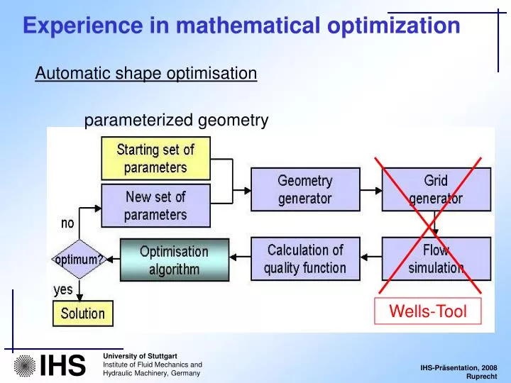
Wells-Tool. Experience in mathematical optimization. Automatic shape optimisation. parameterized geometry. Directe optimisation “Response Surface” method Estimation of an continous approximate function by Neuronal net Polynomial approach Spline

E N D
Wells-Tool Experience in mathematical optimization Automatic shape optimisation parameterized geometry
Directe optimisation “Response Surface” method Estimation of an continous approximate function by Neuronal net Polynomial approach Spline Search for the optimum of the approximate function Optimisation Methods
Response Surface Methode berechnete Werte Qualitätsfunktion Parameter Optimierung an der Response Surface
3 relaxation 1 cost function 2 assumed optimum search direction EXTREME • Gradient type algorithmus, with search direction • Opjective funktion is locally approximated and the minimum is calculated along the search direction
Start with a randomly chosen population New population is obtained by Mutation Crossover Survival of the fittest Live time of each individual is exactly 1 generation (Comma Strategie) Evolution methode Self Adaptive Evolution (SAE)
Research: Asynchronous, parallel optimisation Parallel Optimisation simultaneous simulation on different resources each simulation is run in parallel
Parallel Optimisation Grid Compting
CFD randomly choseninitial parameter sets CFD CFD CFD CFD CFD grid portal CFD CFD CFD Applied Algorithm survival of the fittest new sets by discrete operation, e. g. mirror new sets randomlywith weighting
Geometry Parameterisation Guide vane geometry Inlet angle, Outlet angle, chamber line angle, Weighting factor inlet, Weighting factor outlet, Overlapping,Profile a, Profile b, Trailing edge thickness
Automatic Grid Generation Automatic block structured mesh
Simulation Results: Flow patterns (e. g pressure distribution) Overall quantities (e. g. efficiency, losses) Restrictions (e. g. cavitation) Typical computational time for one geometry: 1-4 hon a Cluster of HPC
Guide vane shape optimized with evolution strategy 9 free parameters: -45 different designs (individuals) per generation -8 generations -in total 360 calculations
Test example: Draft tube cone Din L Dout Assumption:Cone length Optimisation: Outlet diameter
Test example: Draft tube cone Cone length: 6 D_in 1 0.9 0.8 0.7 Draft tube efficiency 0.6 randomly chosen starting points 0.5 0.4 0.6 0.8 1 1.2 1.4 1.6 1.8 2 2.2 2.4 2.6 D_out/D_in
Test example: Draft tube cone 1 0.9 0.8 0.7 Draft tube efficiency 0.6 survivors of the first generation 0.5 0.4 0.6 0.8 1 1.2 1.4 1.6 1.8 2 2.2 2.4 2.6 D_out/D_in
Test example: Draft tube cone 1 0.9 0.8 0.7 Draft tube efficiency 0.6 survivors of the second generation 0.5 0.4 0.6 0.8 1 1.2 1.4 1.6 1.8 2 2.2 2.4 2.6 D_out/D_in
Test example: Draft tube cone 1 0.9 0.8 0.7 Draft tube efficiency 0.6 survivors of the third generation 0.5 0.4 0.6 0.8 1 1.2 1.4 1.6 1.8 2 2.2 2.4 2.6 D_out/D_in
Test example: Draft tube cone 1 0.9 0.8 0.7 Draft tube efficiency 0.6 survivors of the seventh generation computed points 0.5 0.4 0.6 0.8 1 1.2 1.4 1.6 1.8 2 2.2 2.4 2.6 D_out/D_in
Draft tube area distribution Application: Refurbishment of an existing power plant The draft tube contour can only be changed slightly. Optimization of the area distribution
Area distribution represented by B-Spline curves Inlet and outlet kept constant other cross sections scaled up Draft tube area distribution area distribution
Draft tube area distribution Investigated area distribution during the optimisation Design point
Draft tube area distribution Obtained area distribution Design point minimum efficiency original draft tube maximum efficiency draft tube efficiency increase: 8%overall efficiency increase: 0.4%
Draft tube area distribution minimum efficiency design point part load original draft tube Overload