Download
1 / 25
250 likes | 380 Vues
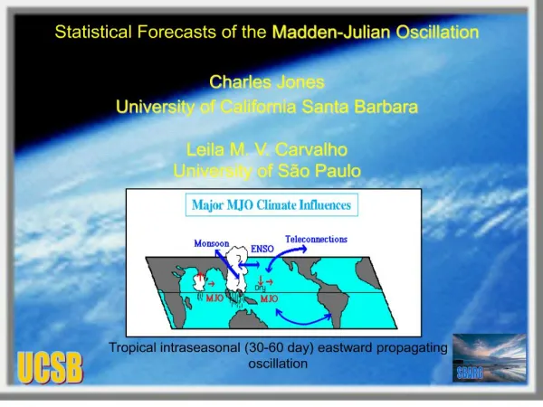
A Homogeneous Stochastic Model of the Madden-Julian Oscillation Charles Jones University of California Santa Barbara. Collaboration : Leila Carvalho (USP ) , A. Matthews (UK) B. Pohl (Fr). Motivations to develop stochastic MJO models.

E N D
A Homogeneous Stochastic Model of the Madden-Julian Oscillation Charles Jones University of California Santa Barbara Collaboration: Leila Carvalho (USP), A. Matthews (UK) B. Pohl (Fr)
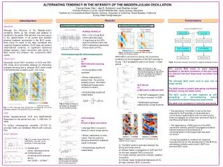
Motivations to develop stochastic MJO models • MJO discovered ~38 years ago; great deal has been learned about the oscillation • However, there are many unresolved issues • Temporal Variability of the MJO Observational knowledge about the MJO is limited to reanalysis data ~60 yrs MJO Weather Climate
Positive trends in MJO intensity (winter and summer) Positive trends in number of MJOs (winter and summer) Jones and Carvalho (2006)
Jones and Carvalho (2006) • Mean winter LF MJO activity: ~uniform variability from 1960s to the mid-1990s • Mean summer LF MJO changes: regime of high activity and low activity during 1958-2004 (~ 18.5 yr)
Long-term changes in MJO activity • what is real signal? • what is data sampling problem? • satellite data • number of raobs
Our Goal: develop stochastic MJO models: • Able to simulate statistical properties of the MJO • Potential to test hypotheses and develop probabilistic approaches to some outstanding MJO issues • Provide additional tools to improve MJO representation in CGCM • Done so far: • homogeneous model • (no seasonal, interannual dependencies)
Typical MJO: 12 34 5 67 8 • Data • Daily U200 and U850 (1948-2006), OLR (1979-2006) • Subtract daily climatology; band-pass filtered (20-200 days) • Average 15S-15N • Combined EOF analysis (U200, U850) • Use (EOF1, PC1), (EOF2, PC2) • Phase angle (PC1,PC2) normalized Wheeler and Hendon (2004)
OLR Anomalies • MJO Identification • Criteria: • Systematic eastward propagation • at least 1 4 • Minimum amplitude: • A = (PC12 + PC22)1/2 > 0.35 • Entire duration between 30-70 days • Mean amplitude during event > 0.9 • 210 MJO events in 1948-2006 Western Pacific 7 6 8 5 West. Hem. & Africa Maritime Continent 1 4 2 3 Indian Ocean
Observed MJO Periods Mean ~46 days Sdv ~10 days Observed MJO Amplitudes A = (PC12 + PC2) 1/2 Mean ~1.50 Sdv ~0.66
Homogeneous Nine States First Order Markov Model 0 Non-MJO MJO 1 8 Western Pacific 81 parameters: 7 6 8 5 etc West. Hem. & Africa 0 Maritime Continent 1 4 2 3 Indian Ocean
Western Pacific MJO starts Eastward propagation 7 6 8 5 Westward propagation 0 Maritime Continent West. Hem. & Africa MJO ends 1 4 Consecutive MJO starts 2 3 Persistence Indian Ocean
Model Simulation • Initial condition S = 0 (non-MJO) • Uniform random number r [0,1] transition probabilities • non-MJO: S=0 MJO: S = [1,2,3,4] • draw random duration Tk days (Gamma PDF fitted to observed MJO durations) • r [0,1]: MJO propagates through phases 1-8 for Tk days • at end of event: S=0 (non-MJO) or S=1 (consecutive MJO) • Given temporal distribution: • phases [1-8] observed composites spatial structure • Intensity: • Amplitude factor: A = 1 + 0.1 R, where R Gaussian number N[0, 1] • Testing: 100 members, each run 59 years
Example of Observed MJO Phase Evolution Example of simulated MJO Phase Evolution
Amplitude factors Simulated MJO Phase Evolution (Example) MJO Phase 0
MJO Simulation Simulation Periods 100 members, 59 years each, 16990 MJOs Mean ~48 days Sdv ~9.3 days Simulation Amplitude Factor 59 year run: 200 MJOs Up to ± 30% weaker/stronger
Number of MJOs per year Observed MJO Ensemble mean
Observations Md ~52 days Sdv ~47.7 days Duration of MJO episodes Simulations Md ~55 days Sdv ~53 days 100 members, 59 years each, 10424 episodes
Observations Md ~60 days Sdv ~85 days Interval between MJO episodes Simulations Md ~90 days Sdv ~125 days 100 members, 59 years each, 10524 intervals
Ratio = 100 x # MJOs simulation # MJOs observations in 59 years (x100)
Wavenumber x Period Spectrum Observations Model
Summary/Conclusions • Homogeneous stochastic model provides a realistic, first order approximation to simulate the main characteristics of the MJO • Model deficiencies: • underestimates total occurrences of MJOs (~20%) • overestimates ratio primary/successive MJOs (x2) • Computation of transition matrix in subsamples: • changes in MJO activity non-homogeneity
Future Work • Non-homogeneous Empirical Model • Time varying transition matrix: • Seasonal variations • Interannual variations (e.g. ENSO state) • Decadal changes (Indian Ocean SSTs ?) • Stochastic model of MJO periods: (Pohl & Matthews 2007) • Interannual variations (ENSO state) • Stochastic model of MJO intensities:(Pohl & Matthews 2007) • Interannual variations (ENSO state) • Decadal changes (before/after ~1977) • Linear trends • www.icess.ucsb.edu/asr