Download
1 / 35
350 likes | 441 Vues
CSE373: Data Structure & Algorithms Lecture 22: More Sorting. Nicki Dell Spring 2014. Admin. Homework 5 partner selection due TODAY! Catalyst link posted on the webpage Homework 5 due next Wednesday at 11pm! Good job for already starting…. The comparison sorting problem.

E N D
CSE373: Data Structure & AlgorithmsLecture 22: More Sorting Nicki Dell Spring 2014
Admin • Homework 5 partner selection due TODAY! • Catalyst link posted on the webpage • Homework 5 due next Wednesday at 11pm! • Good job for already starting…. CSE373: Data Structures & Algorithms
The comparison sorting problem Assume we have n comparable elements in an array and we want to rearrange them to be in increasing order Input: • An array A of data records • A key value in each data record • A comparison function (consistent and total) Effect: • Reorganize the elements of A such that for any i and j, if i < j then A[i] A[j] • (Also, A must have exactly the same data it started with) • Could also sort in reverse order, of course An algorithm doing this is a comparison sort CSE373: Data Structures & Algorithms
Sorting: The Big Picture Surprising amount of neat stuff to say about sorting: Simple algorithms: O(n2) Fancier algorithms: O(n log n) Comparison lower bound: (n log n) Specialized algorithms: O(n) Handling huge data sets Insertion sort Selection sort Shell sort … Heap sort Merge sort Quick sort … Bucket sort Radix sort External sorting CSE373: Data Structures & Algorithms
Divide and conquer Very important technique in algorithm design • Divide problem into smaller parts • Independently solve the simpler parts • Think recursion • Or potential parallelism • Combine solution of parts to produce overall solution CSE373: Data Structures & Algorithms
Divide-and-Conquer Sorting Two great sorting methods are fundamentally divide-and-conquer • Merge sort: Sort the left half of the elements (recursively) Sort the right half of the elements (recursively) Merge the two sorted halves into a sorted whole • Quick sort: Pick a “pivot” element Divide elements into less-than pivot and greater-than pivot Sort the two divisions (recursively on each) Answer is sorted-less-than then pivot then sorted-greater-than CSE373: Data Structures & Algorithms
Quick sort • A divide-and-conquer algorithm • Recursively chop into two pieces • Instead of doing all the work as we merge together, we will do all the work as we recursively split into halves • Unlike merge sort, does not need auxiliary space • O(nlogn) on average , but O(n2) worst-case • Faster than merge sort in practice? • Often believed so • Does fewer copies and more comparisons, so it depends on the relative cost of these two operations! CSE373: Data Structures & Algorithms
Quicksort Overview • Pick a pivot element • Partition all the data into: • The elements less than the pivot • The pivot • The elements greater than the pivot • Recursively sort A and C • The answer is, “as simple as A, B, C” CSE373: Data Structures & Algorithms
Think in Terms of Sets S select pivot value 81 31 57 43 13 75 92 0 26 65 S1 S2 partition S 0 31 75 43 65 13 81 92 26 57 Quicksort(S1) and Quicksort(S2) S1 S2 0 13 26 31 43 57 75 81 92 65 S Presto! S is sorted 0 13 26 31 43 57 65 75 81 92 [Weiss] CSE373: Data Structures & Algorithms
Example, Showing Recursion 8 2 9 4 5 3 1 6 Divide 5 2 4 3 1 8 9 6 Divide 3 8 4 9 2 1 6 Divide 1 Element 1 2 Conquer 1 2 Conquer 6 8 9 1 2 3 4 Conquer 1 2 3 4 5 6 8 9 CSE373: Data Structures & Algorithms
Details Have not yet explained: • How to pick the pivot element • Any choice is correct: data will end up sorted • But as analysis will show, want the two partitions to be about equal in size • How to implement partitioning • In linear time • In place CSE373: Data Structures & Algorithms
Pivots 8 8 2 2 9 9 4 4 5 5 3 3 1 1 6 6 5 1 2 4 3 1 8 2 9 4 5 3 6 8 9 6 • Best pivot? • Median • Halve each time • Worst pivot? • Greatest/least element • Problem of size n - 1 • O(n2) CSE373: Data Structures & Algorithms
Potential pivot rules While sorting arr from lo to hi-1… • Pick arr[lo] or arr[hi-1] • Fast, but worst-case occurs with mostly sorted input • Pick random element in the range • Does as well as any technique, but (pseudo)random number generation can be slow • Still probably the most elegant approach • Median of 3, e.g., arr[lo], arr[hi-1], arr[(hi+lo)/2] • Common heuristic that tends to work well CSE373: Data Structures & Algorithms
Partitioning • Conceptually simple, but hardest part to code up correctly • After picking pivot, need to partition in linear time in place • One approach (there are slightly fancier ones): • Swap pivot with arr[lo] • Use two fingers i and j, starting at lo+1 and hi-1 • while (i < j) if (arr[j] > pivot) j-- else if (arr[i] < pivot) i++ else swap arr[i] with arr[j] • Swap pivot with arr[i] * *skip step 4 if pivot ends up being least element CSE373: Data Structures & Algorithms
Example • Step one: pick pivot as median of 3 • lo = 0, hi = 10 0 1 2 3 4 5 6 7 8 9 8 1 4 9 0 3 5 2 7 6 • Step two: move pivot to the lo position 0 1 2 3 4 5 6 7 8 9 6 1 4 9 0 3 5 2 7 8 CSE373: Data Structures & Algorithms
Example Often have more than one swap during partition – this is a short example Now partition in place Move fingers Swap Move fingers Move pivot 6 1 4 9 0 3 5 2 7 8 6 1 4 9 0 3 5 2 7 8 6 1 4 2 0 3 5 9 7 8 6 1 4 2 0 3 5 9 7 8 5 1 4 2 0 3 6 9 7 8 CSE373: Data Structures & Algorithms
Quick sort visualization • http://www.cs.usfca.edu/~galles/visualization/ComparisonSort.html CSE373: Data Structures & Algorithms
Analysis • Best-case: Pivot is always the median T(0)=T(1)=1 T(n)=2T(n/2) + n -- linear-time partition Same recurrence as merge sort: O(nlogn) • Worst-case: Pivot is always smallest or largest element T(0)=T(1)=1 T(n) = 1T(n-1) + n Basically same recurrence as selection sort: O(n2) • Average-case (e.g., with random pivot) • O(nlogn), not responsible for proof (in text) CSE373: Data Structures & Algorithms
Cutoffs • For small n, all that recursion tends to cost more than doing a quadratic sort • Remember asymptotic complexity is for large n • Common engineering technique: switch algorithm below a cutoff • Reasonable rule of thumb: use insertion sort for n < 10 • Notes: • Could also use a cutoff for merge sort • Cutoffs are also the norm with parallel algorithms • Switch to sequential algorithm • None of this affects asymptotic complexity CSE373: Data Structures & Algorithms
Cutoff pseudocode void quicksort(int[] arr, intlo, inthi) { if(hi – lo < CUTOFF) insertionSort(arr,lo,hi); else … } • Notice how this cuts out the vast majority of the recursive calls • Think of the recursive calls to quicksort as a tree • Trims out the bottom layers of the tree CSE373: Data Structures & Algorithms
How Fast Can We Sort? • Heapsort & mergesort have O(nlogn) worst-case running time • Quicksort has O(nlogn) average-case running time • These bounds are all tight, actually (nlogn) • Comparison sorting in general is (nlogn) • An amazing computer-science result: proves all the clever programming in the world cannot comparison-sort in linear time CSE373: Data Structures & Algorithms
The Big Picture Surprising amount of juicy computer science: 2-3 lectures… Simple algorithms: O(n2) Fancier algorithms: O(n log n) Comparison lower bound: (n log n) Specialized algorithms: O(n) Handling huge data sets Insertion sort Selection sort Shell sort … Heap sort Merge sort Quick sort (avg) … Bucket sort Radix sort External sorting • How??? • Change the model – assume • more than “compare(a,b)” CSE373: Data Structures & Algorithms
Bucket Sort (a.k.a. BinSort) • If all values to be sorted are known to be integers between 1 and K (or any small range): • Create an array of size K • Put each element in its proper bucket (a.k.a. bin) • If data is only integers, no need to store more than a count of how times that bucket has been used • Output result via linear pass through array of buckets • Example: • K=5 • input (5,1,3,4,3,2,1,1,5,4,5) • output: 1,1,1,2,3,3,4,4,5,5,5 CSE373: Data Structures & Algorithms
Visualization • http://www.cs.usfca.edu/~galles/visualization/CountingSort.html CSE373: Data Structures & Algorithms
Analyzing Bucket Sort • Overall: O(n+K) • Linear in n, but also linear in K • (nlogn) lower bound does not apply because this is not a comparison sort • Good when K is smaller (or not much larger) than n • We don’t spend time doing comparisons of duplicates • Bad when K is much larger than n • Wasted space; wasted time during linear O(K) pass • For data in addition to integer keys, use list at each bucket CSE373: Data Structures & Algorithms
Bucket Sort with Data • Example: Movie ratings; scale 1-5;1=bad, 5=excellent • Input= • 5: Casablanca • 3: Harry Potter movies • 5: Star Wars Original Trilogy • 1: Rocky V Rocky V Harry Potter Casablanca Star Wars • Result: 1: Rocky V, 3: Harry Potter, 5: Casablanca, 5: Star Wars • Easy to keep ‘stable’; Casablanca still before Star Wars Most real lists aren’t just keys; we have data Each bucket is a list (say, linked list) To add to a bucket, insert in O(1) (at beginning, or keep pointer to last element) CSE373: Data Structures & Algorithms
Radix sort • Radix = “the base of a number system” • Examples will use 10 because we are used to that • In implementations use larger numbers • For example, for ASCII strings, might use 128 • Idea: • Bucket sort on one digit at a time • Number of buckets = radix • Starting with least significant digit • Keeping sort stable • Do one pass per digit • Invariant: After k passes (digits), the last k digits are sorted • Aside: Origins go back to the 1890 U.S. census CSE373: Data Structures & Algorithms
Example Radix = 10 Input: 478 537 9 721 3 38 143 67 0 1 2 3 4 5 6 7 8 9 721 3 143 537 67 478 38 9 Order now: 721 3 143 537 67 478 38 9 • First pass: • bucket sort by ones digit CSE373: Data Structures & Algorithms
0 1 2 3 4 5 6 7 8 9 Example 721 3 143 537 67 478 38 9 Radix = 10 0 1 2 3 4 5 6 7 8 9 3 9 721 537 38 143 67 478 Order was: 721 3 143 537 67 478 38 9 Order now: 3 9 721 537 38 143 67 478 • Second pass: • stable bucket sort by tens digit CSE373: Data Structures & Algorithms
0 1 2 3 4 5 6 7 8 9 Example 3 9 721 537 38 143 67 478 Radix = 10 0 1 2 3 4 5 6 7 8 9 3 9 38 67 143 478 537 721 Order was: 3 9 721 537 38 143 67 478 Order now: 3 9 38 67 143 478 537 721 • Third pass: • stable bucket sort by 100s digit CSE373: Data Structures & Algorithms
Visualization • http://www.cs.usfca.edu/~galles/visualization/RadixSort.html CSE373: Data Structures & Algorithms
Analysis Input size: n Number of buckets = Radix: B Number of passes = “Digits”: P Work per pass is 1 bucket sort: O(B+n) Total work is O(P(B+n)) Compared to comparison sorts, sometimes a win, but often not • Example: Strings of English letters up to length 15 • Run-time proportional to: 15*(52 + n) • This is less than n log n only if n > 33,000 • Of course, cross-over point depends on constant factors of the implementations • And radix sort can have poor locality properties CSE373: Data Structures & Algorithms
Sorting massive data • Need sorting algorithms that minimize disk/tape access time: • Quicksort and Heapsort both jump all over the array, leading to expensive random disk accesses • Merge sort scans linearly through arrays, leading to (relatively) efficient sequential disk access • Merge sort is the basis of massive sorting • Merge sort can leverage multiple disks Fall 2013 CSE373: Data Structures & Algorithms 33
External Merge Sort • Sort 900 MB using 100 MB RAM • Read 100 MB of data into memory • Sort using conventional method (e.g. quicksort) • Write sorted 100MB to temp file • Repeat until all data in sorted chunks (900/100 = 9 total) • Read first 10 MB of each sorted chuck, merge into remaining 10MB • writing and reading as necessary • Single merge pass instead of log n • Additional pass helpful if data much larger than memory • Parallelism and better hardware can improve performance • Distribution sorts (similar to bucket sort) are also used CSE373: Data Structures & Algorithms
Last Slide on Sorting • Simple O(n2) sorts can be fastest for small n • Selection sort, Insertion sort (latter linear for mostly-sorted) • Good for “below a cut-off” to help divide-and-conquer sorts • O(n log n) sorts • Heap sort, in-place but not stable nor parallelizable • Merge sort, not in place but stable and works as external sort • Quick sort, in place but not stable and O(n2) in worst-case • Often fastest, but depends on costs of comparisons/copies • (nlogn)is worst-case and average lower-bound for sorting by comparisons • Non-comparison sorts • Bucket sort good for small number of possible key values • Radix sort uses fewer buckets and more phases • Best way to sort? It depends! CSE373: Data Structures & Algorithms