Download
1 / 51
510 likes | 662 Vues
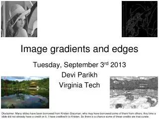
Image gradients and edges. Tuesday, September 3 rd 2013 Devi Parikh Virginia Tech.

E N D
Image gradients and edges Tuesday, September 3rd 2013 Devi Parikh Virginia Tech Disclaimer: Many slides have been borrowed from Kristen Grauman, who may have borrowed some of them from others. Any time a slide did not already have a credit on it, I have credited it to Kristen. So there is a chance some of these credits are inaccurate.
Announcements • Questions? • Everyone was able to add the course? • PS0 was due last night. Slide credit: Devi Parikh
Last time • Image formation • Various models for image “noise” • Linear filters and convolution useful for • Image smoothing, removing noise • Box filter • Gaussian filter • Impact of scale / width of smoothing filter • Separable filters more efficient • Median filter: a non-linear filter, edge-preserving Slide credit: Adapted by Devi Parikh from Kristen Grauman
Review Filter f = 1/9 x [ 1 1 1 1 1 1 1 1 1] f*g=? original image h filtered Slide credit: Kristen Grauman
Review Filter f = 1/9 x [ 1 1 1 1 1 1 1 1 1]T f*g=? original image h filtered Slide credit: Kristen Grauman
Review How do you sharpen an image? Slide credit: Devi Parikh
Review Median filter f: Is f(a+b) = f(a)+f(b)? Example: a = [10 20 30 40 50] b = [55 20 30 40 50] Is f linear? Slide credit: Devi Parikh
Recall: image filtering • Compute a function of the local neighborhood at each pixel in the image • Function specified by a “filter” or mask saying how to combine values from neighbors. • Uses of filtering: • Enhance an image (denoise, resize, etc) • Extract information (texture, edges, etc) • Detect patterns (template matching) Slide credit: Kristen Grauman, Adapted from Derek Hoiem
Edge detection • Goal: map image from 2d array of pixels to a set of curves or line segments or contours. • Why? • Main idea: look for strong gradients, post-process Figure from J. Shotton et al., PAMI 2007 Slide credit: Kristen Grauman
What causes an edge? Depth discontinuity: object boundary Reflectance change: appearance information, texture Cast shadows Change in surface orientation: shape Slide credit: Kristen Grauman
Edges/gradients and invariance Slide credit: Kristen Grauman
intensity function(along horizontal scanline) first derivative edges correspond toextrema of derivative Derivatives and edges An edge is a place of rapid change in the image intensity function. image Slide credit: Svetlana Lazebnik
Derivatives with convolution For 2D function, f(x,y), the partial derivative is: For discrete data, we can approximate using finite differences: To implement above as convolution, what would be the associated filter? Slide credit: Kristen Grauman
Partial derivatives of an image -1 1 1 -1 ? -1 1 or Which shows changes with respect to x? (showing filters for correlation) Slide credit: Kristen Grauman
Assorted finite difference filters >> My = fspecial(‘sobel’); >> outim = imfilter(double(im), My); >> imagesc(outim); >> colormap gray; Slide credit: Kristen Grauman
Image gradient The gradient of an image: The gradient points in the direction of most rapid change in intensity The gradient direction (orientation of edge normal) is given by: The edge strength is given by the gradient magnitude Slide credit: Steve Seitz
Effects of noise Consider a single row or column of the image Plotting intensity as a function of position gives a signal Where is the edge? Slide credit: Steve Seitz
Solution: smooth first Look for peaks in Where is the edge? Slide credit: Kristen Grauman
Derivative theorem of convolution Differentiation property of convolution. Slide credit: Steve Seitz
Derivative of Gaussian filters 0.0030 0.0133 0.0219 0.0133 0.0030 0.0133 0.0596 0.0983 0.0596 0.0133 0.0219 0.0983 0.1621 0.0983 0.0219 0.0133 0.0596 0.0983 0.0596 0.0133 0.0030 0.0133 0.0219 0.0133 0.0030 Slide credit: Kristen Grauman
Derivative of Gaussian filters y-direction x-direction Slide credit: Svetlana Lazebnik
Laplacian of Gaussian Consider Laplacian of Gaussian operator Where is the edge? Zero-crossings of bottom graph Slide credit: Steve Seitz
2D edge detection filters Laplacian of Gaussian Gaussian derivative of Gaussian • is the Laplacian operator: Slide credit: Steve Seitz
Smoothing with a Gaussian Recall: parameter σ is the “scale” / “width” / “spread” of the Gaussian kernel, and controls the amount of smoothing. … Slide credit: Kristen Grauman
Effect of σ on derivatives σ = 1 pixel σ = 3 pixels The apparent structures differ depending on Gaussian’s scale parameter. Larger values: larger scale edges detected Smaller values: finer features detected Slide credit: Kristen Grauman
So, what scale to choose? It depends what we’re looking for. Slide credit: Kristen Grauman
Mask properties • Smoothing • Values positive • Sum to 1 constant regions same as input • Amount of smoothing proportional to mask size • Remove “high-frequency” components; “low-pass” filter • Derivatives • ___________ signs used to get high response in regions of high contrast • Sum to ___ no response in constant regions • High absolute value at points of high contrast Slide credit: Kristen Grauman
Seam carving: main idea [Shai & Avidan, SIGGRAPH 2007] Slide credit: Kristen Grauman
Seam carving: main idea Content-aware resizing Traditional resizing [Shai & Avidan, SIGGRAPH 2007] Slide credit: Kristen Grauman
Seam carving: main idea Slide credit: Devi Parikh
Seam carving: main idea Content-aware resizing • Intuition: • Preserve the most “interesting” content • Prefer to remove pixels with low gradient energy • To reduce or increase size in one dimension, remove irregularly shaped “seams” • Optimal solution via dynamic programming. Slide credit: Kristen Grauman
Seam carving: main idea • Want to remove seams where they won’t be very noticeable: • Measure “energy” as gradient magnitude • Choose seam based on minimum total energy path across image, subject to 8-connectedness. Slide credit: Kristen Grauman
Seam carving: algorithm s1 s2 Let a vertical seam s consist of h positions that form an 8-connected path. Let the cost of a seam be: Optimal seam minimizes this cost: Compute it efficiently with dynamic programming. s3 s4 s5 Slide credit: Kristen Grauman
How to identify the minimum cost seam? • How many possible seams are there? • First, consider a greedy approach: Energy matrix (gradient magnitude) Slide credit: Adapted by Devi Parikh from Kristen Grauman
Seam carving: algorithm If I tell you the minimum cost over all seams starting at row 1 and ending at this point For every pixel in this row: M(i,j) What is the minimum cost over all seams starting at row 1 and ending here? Slide credit: Devi Parikh
Seam carving: algorithm • Compute the cumulative minimum energy for all possible connected seams at each entry (i,j): • Then, min value in last row of M indicates end of the minimal connected vertical seam. • Backtrack up from there, selecting min of 3 above in M. j-1 j j+1 row i-1 j row i Energy matrix (gradient magnitude) M matrix: cumulative min energy (for vertical seams) Slide credit: Kristen Grauman
Example Energy matrix (gradient magnitude) M matrix (for vertical seams) Slide credit: Kristen Grauman
Example Energy matrix (gradient magnitude) M matrix (for vertical seams) Slide credit: Kristen Grauman
Real image example Energy Map Original Image Blue = low energy Red = high energy Slide credit: Kristen Grauman
Real image example Slide credit: Kristen Grauman
Other notes on seam carving • Analogous procedure for horizontal seams • Can also insert seams to increase size of image in either dimension • Duplicate optimal seam, averaged with neighbors • Other energy functions may be plugged in • E.g., color-based, interactive,… • Can use combination of vertical and horizontal seams Slide credit: Kristen Grauman
Example results from students at UT Austin Results from Eunho Yang Slide credit: Kristen Grauman
Results from Suyog Jain Slide credit: Kristen Grauman
Conventional resize Original image Seam carving result Results from Martin Becker Slide credit: Kristen Grauman
Conventional resize Original image Seam carving result Results from Martin Becker Slide credit: Kristen Grauman
Conventional resize (399 by 599) Original image (599 by 799) Seam carving (399 by 599) Results from Jay Hennig Slide credit: Kristen Grauman
Removal of a marked object Results from Donghyuk Shin Slide credit: Kristen Grauman
Removal of a marked object Results from Eunho Yang Slide credit: Kristen Grauman
“Failure cases” with seam carving By Donghyuk Shin Slide credit: Kristen Grauman
“Failure cases” with seam carving By Suyog Jain Slide credit: Kristen Grauman