Download

1 / 41
420 likes | 561 Vues
First-Cut Techniques. Lecturer: Jing Liu Email: neouma@mail.xidian.edu.cn Homepage: http://see.xidian.edu.cn/faculty/liujing Xidian Homepage: http://web.xidian.edu.cn/liujing. First-Cut Techniques. The Greedy Approach Graph Traversal.

E N D
First-Cut Techniques Lecturer: Jing Liu Email: neouma@mail.xidian.edu.cn Homepage: http://see.xidian.edu.cn/faculty/liujing Xidian Homepage: http://web.xidian.edu.cn/liujing
First-Cut Techniques • The Greedy Approach • Graph Traversal • A common characteristic of both greedy algorithms and graph traversal is that they are fast, as they involve making local decisions.
The Greedy Approach • As in the case of dynamic programming algorithms, greedy algorithms are usually designed to solve optimization problems in which a quantity is to be minimized or maximized. • Unlike dynamic programming algorithms, greedy algorithms typically consist of a n iterative procedure that tries to find a local optimal solution. • In some instances, these local optimal solutions translate to global optimal solutions. In others, they fail to give optimal solutions.
The Greedy Approach • A greedy algorithm makes a correct guess on the basis of little calculation without worrying about the future. Thus, it builds a solution step by step. Each step increases the size of the partial solution and is based on local optimization. • The choice make is that which produces the largest immediate gain while maintaining feasibility. • Since each step consists of little work based on a small amount of information, the resulting algorithms are typically efficient.
The Fractional Knapsack Problem • Given n items of sizes s1, s2, …, sn, and values v1, v2, …, vn and size C, the knapsack capacity, the objective is to find nonnegative real numbers x1, x2, …, xn that maximize the sum subject to the constraint
The Fractional Knapsack Problem • This problem can easily be solved using the following greedy strategy: • For each item compute yi=vi/si, the ratio of its value to its size. • Sort the items by decreasing ratio, and fill the knapsack with as much as possible from the first item, then the second, and so forth. • This problem reveals many of the characteristics of a greedy algorithm discussed above: The algorithm consists of a simple iterative procedure that selects that item which produces that largest immediate gain while maintaining feasibility.
The Shortest Path Problem • Let G=(V, E) be a directed graph in which each edge has a nonnegative length, and a distinguished vertex s called the source. The single-source shortest path problem, or simply the shortest path problem, is to determine the distance from s to every other vertex in V,where the distance from vertex s to vertex x is defined as the length of a shortest path from s to x. • For simplicity, we will assume that V={1, 2, …, n} and s=1. • This problem can be solved using a greedy technique known as Dijkstra’s algorithm.
The Shortest Path Problem • The set of vertices is partitioned into two sets X and Y so that X is the set of vertices whose distance from the source has already been determined, while Y contains the rest vertices. Thus, initially X={1} and Y={2, 3, …, n}. • Associated with each vertex y in Y is a label [y], which is the length of a shortest path that passes only through vertices in X. Thus, initially
The Shortest Path Problem • At each step, we select a vertex yY with minimum and move it to X, and of each vertex wY that is adjacent to y is updated indicating that a shorter path to w via y has been discovered. • The above process is repeated until Y is empty. • Finally, of each vertex in X is the distance from the source vertex to this one.
The Shortest Path Problem • Example: 3 2 4 1 15 9 4 6 1 13 4 12 5 3 5
The Shortest Path Problem • Input: A weighted directed graph G=(V, E), where V={1, 2, …, n}; • Output: The distance from vertex 1 to every other vertex in G; • 1. X={1}; YV-{1}; [1]0; • 2. for y2 to n • 3. if y is adjacent to 1 then [y]length[1, y]; • 4. else [y]; • 5. end if; • 6. end for; • 7. for j1 to n-1 • 8. Let yY be such that [y] is minimum; • 9. XX{y}; //add vertex y to X • 10. YY-{y}; //delete vertex y from Y • 11. for each edge (y, w) • 12. if wY and [y]+length[y, w]<[w] then • 13. [w][y]+length[y, w]; • 14. end for; • 15. end for;
The Shortest Path Problem • What’s the performance of the DIJKSTRA algorithm? • Time Complexity?
The Shortest Path Problem • Given a directed graph G with nonnegative weights on its edges and a source vertex s, Algorithm DIJKSTRA finds the length of the distance from s to every other vertex in (n2) time.
The Shortest Path Problem • Write codes to implement the Dijkstra algorithm.
Minimum Cost Spanning Trees (Kruskal’s Algorithm) • Let G=(V, E) be a connected undirected graph with weights on its edges. • A spanning tree (V, T) of G is a subgraph of G that is a tree. • If G is weighted and the sum of the weights of the edges in T is minimum, then (V, T) is called a minimum cost spanning tree or simply a minimum spanning tree.
Minimum Cost Spanning Trees (Kruskal’s Algorithm) • Kruskal’s algorithm works by maintaining a forest consisting of several spanning trees that are gradually merged until finally the forest consists of exactly one tree. • The algorithm starts by sorting the edges in nondecreasing order by weight.
Minimum Cost Spanning Trees (Kruskal’s Algorithm) • Next, starting from the forest (V, T) consisting of the vertices of the graph and none of its edges, the following step is repeated until (V, T) is transformed into a tree: Let (V, T) be the forest constructed so far, and let eE-T be the current edge being considered. If adding e to T does not create a cycle, then include e in T; otherwise discard e. • This process will terminate after adding exactly n-1 edges.
Minimum Cost Spanning Trees (Kruskal’s Algorithm) • Example: 11 2 4 1 3 6 9 6 1 7 4 2 13 3 5
Minimum Cost Spanning Trees (Kruskal’s Algorithm) • Write codes to implement the Kruskal algorithm.
File Compression • Suppose we are given a file, which is a string of characters. We wish to compress the file as much as possible in such a way that the original file can easily be reconstructed. • Let the set of characters in the file be C={c1, c2, …, cn}. Let also f(ci), 1in, be the frequency of character ci in the file, i.e., the number of times ci appears in the file.
File Compression • Using a fixed number of bits to represent each character, called the encoding of the character, the size of the file depends only on the number of characters in the file. • Since the frequency of some characters may be much larger than others, it is reasonable to use variable length encodings.
File Compression • Intuitively, those characters with large frequencies should be assigned short encodings, whereas long encodings may be assigned to those characters with small frequencies. • When the encodings vary in length, we stipulate that the encoding of one character must not be the prefix of the encoding of another character; such codes are called prefix codes. • For instance, if we assign the encodings 10 and 101 to the letters “a” and “b”, there will be an ambiguity as to whether 10 is the encoding of “a” or is the prefix of the encoding of the letter “b”.
File Compression • Once the prefix constraint is satisfied, the decoding becomes unambiguous; the sequence of bits is scanned until an encoding of some character is found. • One way to “parse” a given sequence of bits is to use a full binary tree, in which each internal node has exactly two branches labeled by 0 an 1. The leaves in this tree corresponding to the characters. Each sequence of 0’s and 1’s on a path from the root to a leaf corresponds to a character encoding.
File Compression • The algorithm presented is due to Huffman. • The algorithm consists of repeating the following procedure until C consists of only one character. • Let ci and cj be two characters with minimum frequencies. • Create a new node c whose frequency is the sum of the frequencies of ci and cj, and make ci and cj the children of c. • Let C=C-{ci, cj}{c}.
File Compression • Example: C={a, b, c, d, e} f (a)=20 f (b)=7 f (c)=10 f (d)=4 f (e)=18
Graph Traversal • In some cases, what is important is that the vertices are visited in a systematic order, regardless of the input graph. Usually, there are two methods of graph traversal: • Depth-first search • Breadth-first search
Depth-First Search • Let G=(V, E) be a directed or undirected graph. • First, all vertices are marked unvisited. • Next, a starting vertex is selected, say vV, and marked visited. Let w be any vertex that is adjacent to v. We mark w as visited and advance to another vertex, say x, that is adjacent to w and is marked unvisited. Again, we mark x as visited and advance to another vertex that is adjacent to x and is marked unvisited.
Depth-First Search • This process of selecting an unvisited vertex adjacent to the current vertex continues as deep as possible until we find a vertex y whose adjacent vertices have all been marked visited. • At this point, we back up to the most recently visited vertex, say z, and visit an unvisited vertex that is adjacent to z, if any. • Continuing this way, we finally return back to the starting vertex v. • The algorithm for such a traversal can be written using recursion.
Depth-First Search • Example: a d i c b g h e f j
Depth-First Search • When the search is complete, if all vertices are reachable from the start vertex, a spanning tree called the depth-first search spanning tree is constructed whose edges are those inspected in the forward direction, i.e., when exploring unvisited vertices. • As a result of the traversal, the edges of an undirected graph G are classified into the following two types: • Tree edges: edges in the depth-first search tree. • Back edges: all other edges.
Depth-First Search • Input: An undirected graph G=(V, E); • Output: Preordering of the vertices in the corresponding depth-first search tree. • 1. predfn0; • 2. for each vertex vV • 3. Mark v unvisited; • 4. end for; • 5. for each vertex vV • 6. if v is marked unvisited then dfs(v); • 7. end for; • dfs(v) • 1. Mark v visited; • 2. predfnpredfn+1; • 3. for each edge (v, w)E • 4. if w is marked unvisited then dfs(w); • 5. end for;
Depth-First Search • Write codes to implement the Depth-First Search on graph.
Breadth-First Search • When we visit a vertex v, we next visit all vertices adjacent to v. • This method of traversal can be implemented by a queue to store unexamined vertices.
Finding Articulation Points in a Graph • A vertex v in an undirected graph G with more than two vertices is called an articulation point if there exist two vertices u and w different from v such that any path between u and w must pass through v. • If G is connected, the removal of v and its incident edges will result in a disconnected subgraph of G. • A graph is called biconnected if it is connected and has no articulation points.
Finding Articulation Points in a Graph • To find the set of articulation points, we perform a depth-first search traversal on G. • During the traversal, we maintain two labels with each vertex vV: [v] and [v]. • [v] is simply predfn in the depth-first search algorithm. [v] is initialized to [v], but may change later on during the traversal.
Finding Articulation Points in a Graph • For each vertex v visited, we let [v] be the minimum of the following: • [v] • [u] for each vertex u such that (v, u) is a back edge • [w] for each vertex w such that (v, w) is a tree edge Thus, [v] is the smallest that v can reach through back edges or tree edges.
Finding Articulation Points in a Graph The articulation points are determined as follows: • The root is an articulation point if and only if it has two or more children in the depth-first search tree. • A vertex v other than the root is an articulation point if and only if v has a child w with [w][v].
Finding Articulation Points in a Graph • Input: A connected undirected graph G=(V, E); • Output: Array A[1…count] containing the articulation points of G, if any. • 1. Let s be the start vertex; • 2. for each vertex vV • 3. Mark v unvisited; • 4. end for; • 5. predfn0; count0; rootdegree0; • 6. dfs(s);
dfs(v) • 1. Mark v visited; artpointfalse; predfnpredfn+1; • 2. [v]predfn; [v]predfn; • 3. for each edge (v, w)E • 4. if (v, w) is a tree edge then • 5. dfs(w); • 6. if v=s then • 7. rootdegreerootdegree+1; • 8. if rootdegree=2 then artpointtrue; • 9. else • 10. [v]min{[v], [w]}; • 11. if [w][v] then artpointtrue; • 12. end if; • 13. else if (v, w) is a back edge then [v]min{[v], [w]}; • 14. else do nothing; //w is the parent of v • 15. end if; • 16. end for; • 17. if artpoint then • 18. countcount +1; • 19. A[count]v; • 20. end if;
Finding Articulation Points in a Graph • Example: a d i c b g h e f j
Finding Articulation Points in a Graph • Write codes to implement the above algorithm.