Download
1 / 118
1.34k likes | 1.76k Vues
9 – Stereo Reconstruction. Slides from A. Zisserman & S. Lazebnik. Overview. Single camera geometry Recap of Homogenous coordinates Perspective projection model Camera calibration Stereo Reconstruction Epipolar geometry Stereo correspondence Triangulation. Single camera geometry.

E N D
9 – Stereo Reconstruction Slides from A. Zisserman & S. Lazebnik
Overview • Single camera geometry • Recap of Homogenous coordinates • Perspective projection model • Camera calibration • Stereo Reconstruction • Epipolar geometry • Stereo correspondence • Triangulation
X? X? X? Projective Geometry • Recovery of structure from one image is inherently ambiguous • Today focus on geometry that maps world to camera image x
Recall: Pinhole camera model • Principal axis: line from the camera center perpendicular to the image plane • Normalized (camera) coordinate system: camera center is at the origin and the principal axis is the z-axis
Recap: Homogeneous coordinates • Is this a linear transformation? • Trick: add one more coordinate: • no—division by z is nonlinear homogeneous scene coordinates homogeneous image coordinates Converting from homogeneous coordinates Slide by Steve Seitz
Principal point • Principal point (p): point where principal axis intersects the image plane (origin of normalized coordinate system) • Normalized coordinate system: origin is at the principal point • Image coordinate system: origin is in the corner • How to go from normalized coordinate system to image coordinate system?
Principal point offset principal point:
Principal point offset principal point: calibration matrix
Pixel coordinates • mx pixels per meter in horizontal direction, my pixels per meter in vertical direction Pixel size: m pixels pixels/m
Camera rotation and translation • In general, the camera coordinate frame will be related to the world coordinate frame by a rotation and a translation coords. of point in camera frame coords. of camera center in world frame coords. of a pointin world frame (nonhomogeneous)
Camera rotation and translation In non-homogeneouscoordinates: Note: C is the null space of the camera projection matrix (PC=0)
Camera parameters • Intrinsic parameters • Principal point coordinates • Focal length • Pixel magnification factors • Skew (non-rectangular pixels) • Radial distortion
Camera parameters • Intrinsic parameters • Principal point coordinates • Focal length • Pixel magnification factors • Skew (non-rectangular pixels) • Radial distortion • Extrinsic parameters • Rotation and translation relative to world coordinate system
Xi xi Camera calibration • Given n points with known 3D coordinates Xi and known image projections xi, estimate the camera parameters
Camera calibration Two linearly independent equations
Camera calibration • P has 11 degrees of freedom (12 parameters, but scale is arbitrary) • One 2D/3D correspondence gives us two linearly independent equations • Homogeneous least squares • 6 correspondences needed for a minimal solution
Camera calibration • Note: for coplanar points that satisfy ΠTX=0,we will get degenerate solutions (Π,0,0), (0,Π,0), or (0,0,Π)
Camera calibration • Once we’ve recovered the numerical form of the camera matrix, we still have to figure out the intrinsic and extrinsic parameters • This is a matrix decomposition problem, not an estimation problem (see F&P sec. 3.2, 3.3)
Alternative: multi-plane calibration Images courtesy Jean-Yves Bouguet, Intel Corp. • Advantage • Only requires a plane • Don’t have to know positions/orientations • Good code available online! • Intel’s OpenCV library:http://www.intel.com/research/mrl/research/opencv/ • Matlab version by Jean-Yves Bouget: http://www.vision.caltech.edu/bouguetj/calib_doc/index.html • Zhengyou Zhang’s web site: http://research.microsoft.com/~zhang/Calib/ Projective Geometry
known camera viewpoints Shape (3D) from two (or more) images Stereo Reconstruction
Example images shape surface reflectance
Scenarios The two images can arise from • A stereo rig consisting of two cameras • the two images are acquired simultaneously or • A single moving camera (static scene) • the two images are acquired sequentially The two scenarios are geometrically equivalent
Stereo head Camera on a mobile vehicle
The objective Giventwo images of a scene acquired by known cameras compute the 3D position of the scene (structure recovery) • Basic principle:triangulate from corresponding image points • Determine 3D point at intersection of two back-projected rays
/ C Corresponding points are images of the same scene point Triangulation C The back-projected points generate rays which intersect at the 3D scene point
An algorithm for stereo reconstruction • For each point in the first image determine the corresponding point in the second image • (this is a search problem) • For each pair of matched points determine the 3D point by triangulation • (this is an estimation problem)
The correspondence problem Givena point x in one image find the corresponding point in the other image This appears to be a 2D search problem, but it is reduced to a 1D search by the epipolar constraint
Outline • Epipolar geometry • the geometry of two cameras • reduces the correspondence problem to a line search • Stereo correspondence algorithms • Triangulation
/ C Notation The two cameras are P and P/, and a 3D point X is imaged as X P P/ x / x C Warning for equations involving homogeneous quantities ‘=’means ‘equal up to scale’
? epipolarline / C epipole baseline Epipolar geometry Given an image point in one view, where is the corresponding point in the other view? C • A point in one view “generates” an epipolarline in the other view • The corresponding point lies on this line
Epipolar line • Epipolar constraint • Reduces correspondence problem to 1D search along an epipolar line
/ C Epipolar geometry continued Epipolar geometry is a consequence of the coplanarity of the camera centres and scene point X x / x C The cameracentres, corresponding points and scene point lie in a single plane, known as the epipolar plane
/ C Nomenclature X l/ right epipolar line left epipolar line x / x e / e C • The epipolar linel/ is the image of the ray through x • The epipole e is the point of intersection of the line joining the camera centres with the image plane • this line is the baseline for a stereo rig, and • the translation vector for a moving camera • The epipole is the image of the centre of the other camera: e = PC/ , e/ = P/C
/ e The epipolar pencil X e baseline As the position of the 3D point X varies, the epipolar planes “rotate” about the baseline. This family of planes is known as an epipolar pencil. All epipolar lines intersect at the epipole. (a pencil is a one parameter family)
/ e The epipolar pencil X e baseline As the position of the 3D point X varies, the epipolar planes “rotate” about the baseline. This family of planes is known as an epipolar pencil. All epipolar lines intersect at the epipole. (a pencil is a one parameter family)
Epipolar geometry example I: parallel cameras Epipolar geometry depends only on the relative pose (position and orientation) and internal parameters of the two cameras, i.e. the position of the camera centres and image planes. It does not depend on the scene structure (3D points external to the camera).
/ e Epipolar geometry example II: converging cameras e Note, epipolar lines are in general not parallel
The line l through the two points p and q is l = p x q Proof • The intersection of two lines l and m is the point x = l x m Example: compute the point of intersection of the two lines l and m in the figure below y l 1 m 2 x which is the point (2,1)
Algebraic representation of epipolar geometry We know that the epipolar geometry defines a mapping x l/ point in first image epipolar line in second image
Derivation of the algebraic expression Outline P Step 1: for a point x in the first image back project a ray with camera P P/ Step 2: choose two points on the ray and project into the second image with camera P/ Step 3: compute the line through the two image points using the relation l/ = p x q
choose camera matrices internal calibration rotation translation from world to camera coordinate frame • first camera world coordinate frame aligned with first camera • second camera
Step 1: for a point x in the first image back project a ray with camera P A point x back projects to a ray where Z is the point’s depth, since satisfies