Download
1 / 57
570 likes | 731 Vues
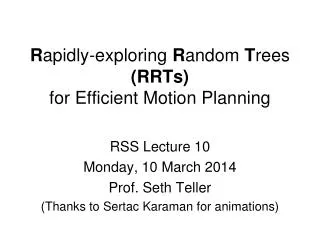
R apidly-exploring R andom T rees (RRTs) for Efficient Motion Planning. RSS Lecture 10 Mon day , 10 March 2014 Prof. Seth Teller (Thanks to Sertac Karaman for animations). Recap of Previous Lectures:. Recall the motion planning problem: We discussed: Cell decomposition

E N D
Rapidly-exploring Random Trees (RRTs)for Efficient Motion Planning RSS Lecture 10 Monday, 10 March 2014 Prof. Seth Teller (Thanks to SertacKaraman for animations)
Recap of Previous Lectures: • Recall the motion planning problem: • We discussed: • Cell decomposition • Guided search using A* • Potential fields • Configuration space • Probabilistic Road Maps
Recap: PRMs [Kavraki et al. 1996] goal 1. Randomly generate robot configurations (nodes) - Discard invalid nodes (how?) 2. Connect pairs of nodes to form roadmap edges - Use simple, deterministic local planner - Discard invalid edges (how?) Plan Generation (Query processing) start 1. Link start and goalposes into roadmap 2. Find path fromstarttogoal within roadmap3. Generate motion plan for each edge used C-space Roadmap Construction (Pre-processing) C-obst C-obst C-obst C-obst C-obst • Primitives Required: • Method for sampling C-Space points • Method for “validating” C-space points and edges
Today’s Focus • Retain assumptions: • Perfect map • Perfect localization • Incorporate additional elements: • Unstabledynamics • Cars, helicopters, humanoids, … • Agile maneuvering aircraft • High-dimensionalconfiguration space • Real-time and online • Trajectory design & execution
Today’s Focus • Retain assumptions: • Perfect map • Perfect localization • Incorporate additional elements: • Unstabledynamics • Cars, helicopters, humanoids, … • Agile maneuvering aircraft • High-dimensionalconfiguration space • Real-time and online • Trajectory design & execution
Today’s Focus • Retain assumptions: • Perfect map • Perfect localization • Incorporate additional elements: • Unstabledynamics • Cars, helicopters, humanoids, … • Agile maneuvering aircraft • High-dimensionalconfiguration space • Real-time and online • Trajectory generation & execution
Motion Planning Revisited • Given: • Robot's dynamics • A map of the environment (perfect information, but discovered online) • Robot's pose in the map • A goal pose in the map • Find a sequence of • Actuation commands (such as steer, gas/brake, transmission) • In real time (requires efficient algorithms) … that drive system to the goal pose • Problem is essential in almost all robotics applications irrespective of size, type of actuation, sensor suite, task domain, etc.
Practical Challenges • Safety: do not collide with anything; • ensure that system is stable; etc. • Computational effectiveness: problem is (provably) computa-tionally very challenging • Optimize: fuel, efficiency etc. • Social challenges (in human-occupied environments): motion should seem natural; robot should be accepted by humans
Practical Challenges • Safety: do not collide with anything; • ensure that system is stable; etc. • Computational effectiveness: problem is (provably) computa-tionallyvery challenging • Optimize: fuel, efficiency etc. • Social challenges (in human-occupied environments): motion should seem natural;robot should be accepted by humans
Practical Challenges • Safety: do not collide with anything; • ensure that system is stable; etc. • Computational effectiveness:problem is (provably) computa-tionallyvery challenging • Optimality: fuel, efficiency etc.(alternative framing: not a gross waste of resources) • Social acceptability (in human-occupied environments):motion should seem natural;robot’s presence should not be rejected by humans
Practical Challenges • Safety: do not collide with anything; • ensure that system is stable; etc. • Computational effectiveness:problem is (provably) computa-tionallyvery challenging • Optimize: fuel, efficiency etc.(alternative framing: not a gross waste of resources) • Social acceptability (in human-occupied environments): motion should seem natural;robot’s presence should not be rejected by humans
Different Approaches • Algebraic Planners • Cell Decomposition • Potential Fields • Sampling-Based Methods
Motion Planning Approaches • Algebraic Planners • Explicit (algebraic) representation of obstacles • Use algebraic expressions (of visibility comp-utations, projections etc.) to find the path • Complete (finds a solution if one exists, otherwise reports failure) • Computationally very intensive – impractical • Cell Decomposition • Potential Fields. • Sampling-Based Methods 1. Represent with polynomial inequalities 2. Transform inequalities to c-space 3. Solve inequalities in c-space to check feasibility and find a plan
Motion Planning Approaches • Algebraic Planners • Cell Decomposition • Analytic methods don’t scale well withdimension (too many cells in high d) • Gridding methods are only “resolution complete” (i.e., will find a solution onlyif the grid resolution is fine enough, and if enough grid cells are inspected) • Potential Fields. • Sampling-Based Methods Analytic subdivision Gridded subdivision
Motion Planning Approaches • Algebraic Planners • Cell Decomposition • Potential Fields • No completeness guarantee (can get stuck in local minima) • Of intermediate efficiency; don’t handle dynamic environments well • Sampling-Based Methods
Motion Planning Approaches goal • Algebraic Planners • Cell Decomposition • Potential Fields • Sampling-Based Methods • (Randomly) construct a set of feasible (that is, collision-free) trajectories • “Probabilistically complete” (if run longenough, very likely to find a solution) • Quite efficient; methods scale well with increasing dimension, # of obstacles C-obst C-obst C-obst C-obst C-obst goal start
Sampling Strategies • How can we draw random samples from within c-space? • Normalize all c-space dimensions to lie inside [0..1] • Then, simple idea: • Generate a random point in d-dimensional space • Independently generate d random numbers between 0 and 1 • Aggregate all d numbers into a single point in c-space 2. Check whether sample point (i.e., robot pose) lies within any obstacle
Example Sample Sets Uniform sampling: From a given axis, sample each coordinate with equal likelihood (200 random samples) (200 random samples) Observe: Significant local variation, but sample sets are globally consistent (Later, we’ll see that this yields consistent performance across runs)
Sampling-based Motion Planning • Basic idea: • Randomly sample n points from c-space • Connect them to each other (if no collision with obstacles) • Recall the two primitive procedures: • Check if a point is in the obstacle-free space • Check if a trajectory lies in the obstacle-free space This is the Probabilistic Road Map (PRM) algorithm goal C-obst C-obst C-obst PRM is a multiple-queryalgorithm (can reuse the roadmap for many queries) C-obst C-obst goal start
IncrementalSampling-based Motion Planning • Sometimes building a roadmap a priori might be inefficient (or even impractical) • Assumes that all regions of c-spacewill be utilized during actual motions • Building a roadmap requires global knowledge • But in real settings, obstacles are not known a priori; rather, they are discovered online • We desire an incremental method: • Generate motion plans for a single start, goal pose • Expending more CPU yields better motion plans • The Rapidly-exploring Random Tree (RRT) algorithm meets these requirements
RRT Data Structure, Algorithm T = (nodes V, edges E): tree structure • Initialized as single root vertex (the robot’s current pose) RRTroot // Sample a node x from c-space // Find nearest node v in tree // Extend nearest node toward sample // If extension is collision-free ; // Add new node and edge to tree
Digression: Voronoi Diagrams Given nsites in d dimensions, the Voronoi diagram of the sites is a partition of Rd into regions, one region per site, such that all points in the interior of each region lie closer to that region’s site than to any other site (AKA Dirichlettesselations, Wigner-Seitz regions, Thiessen polygons, Brillouinzones, …)
Rapidly-exploring Random Trees:Clearly random! Why rapidly-exploring? • RRTs tend to grow toward unexplored portions of the state-space • Unexplored regions are (in some sense) more likely to be sampled • This is called a Voronoi bias For an RRT at a given iteration, some nodesare associated with large Voronoi regions ofc-space, some with smaller Voronoi regions The unexplored areas of c-space tend tocoincide with the larger Voronoi regions (Uniform) samples will tend to fall intorelatively larger Voronoi regions Thus unexplored regions will tend to shrink! Main advantage of RRT: Samples “grow” tree toward unexplored regions of c-space!
Rapidly-exploring Random Treesin simulation Goal pose region Initial pose Obstacles The tree Best path in the tree (identifiedthrough search)
Rapidly-exploring Random Treesin simulation Movie shows the RRT exploring empty c-space Goal pose region
Rapidly-exploring Random Treesin simulation Exploration amid obstacles, narrow passages:
Performance of Sampling-based Methods • Why do the PRM and RRT methods work so well? • Probabilistic Completeness: • The probability that the RRT will find a path approaches 1 as the number of samples increases — if a feasible path exists. • The approach rate is exponential —if the environment has good “visibility’’ properties • ϵ-goodness: • A point is ϵ-good if it “sees” at least an ϵ fraction of the obstacle-free space • An environment is ϵ-good if all freespace points in it are ϵ-good Good performance of PRMs and RRTs has been tied to the fact that, in practice, most applications feature environments with good visibility guarantees (Latombe et al., IJRR ’06).
Example: Unmanned Driving Goal pose • Tree of trajectories is grown by sampling configurations randomly • Rapidly explores several configurations that the robot can reach. • Many test trajectories generated(tens of thousands per second) • Safety of any trajectory is “guaranteed”… • … as of instantaneous world stateat the time of trajectory generation • Choose best one that reaches the goal, e.g., • Maximizes minimum distance to obstacles • Minimizes total path length • Supports dynamic replanning; if current trajectory becomes infeasible: • Choose another one that is feasible • If none remain, then E-stop Obstacleinfeasible Lane divider undesirable Road infeasible Vehicle
Real-world Implementation A few details: • CPU limitations and sampling method • Dynamical feasibility constraints • Grid map with local obstacle awareness • Stop nodes for safety Legend for images, videos you’ll see next: Instantaneous vehicle pose Reaching, low cost Obstacle Reaching, high cost High-cost regions Non-reaching Goal pose
Summary • The Rapidly-exploring Random Tree (RRT) algorithm • Discussed challenges for motion planning methods in real-world applications • Intuition behind good performance of sampling-based methods • Two applications: • Urban Challenge vehicle, Agile Robotics forklift
For next year • Better image choices pp. 29-32 • Make grid scaling discussionmore explicit
System Architecture • System has 40 CPUs, 70+ processes • Processes communicate with each other only via message passing • The core planning and control processes and some components that they are directly connected to Checkpoints Road network Navigator Obstacle Map Planner (RRT) Controller Vehicle
Dynamical Feasibility • Vehicle (car, forklift) is modeled as a dynamical system with 5 states: • X • Y • Theta (heading) • Speed • Sideslip – not used for planning • A closed-loop controller is designed to stabilize the system in • Position/orientation (X, Y, Theta) • Speed control • The RRT samples controller setpoints(which a lower-level controller then tracks) • This process ensures dynamical feasibility (i.e. generates only trajectories that can indeed be executed by the vehicle)
Grid Map and Moving Obstacles • The RRT uses the grid map data structure,which provides one efficient query: • Check whether a specified hypothetical trajectory collideswith any (dilated) obstacle • The perception subsystem also detects moving obstacles and predicts their future trajectories Checkpoints Road network Navigator Obstacle Map Planner (RRT) Controller Vehicle
Stop Nodes • Remember the safety requirement. • All leaf nodes constrained to have speed=0 • The RRT attempts to maintain a path from every internal node to some leaf node • If, due to some newly discovered obstacle,no such trajectory exists in the tree, the robot “E-stops” (i.e., slams on the brakes) • Safety is perhaps the most important requirement in real-time motion planning for robotic vehicles.
Sampling Strategies No labels for lasttwo images?? • Measuring the “quality” of samples: Dispersion methods How good is uniform sampling? How about deterministic methods?
Rapidly-exploring Random Treesin simulation A linear dynamical system with 2 states and drift:
Limitations of RRT • RRT algorithm is tailored to find a feasible solution very quickly.
Limitations of RRT • RRT algorithm is tailored to find a feasible solution very quickly. • However, our simulation results suggest that, if kept running, the solution is not improved in terms of quality.
Limitations of RRT • RRT algorithm is tailored to find a feasible solution very quickly. • However, our simulation results suggest that, if kept running, the solution is not improved in terms of quality. • Can we formalize this claim? • Let s* be an optimal path and c* denote its cost. • Let Xn be a random variable that denotes the cost of the best path in the RRT at the end of iteration n. • That is, the probability that RRT will get closer to an optimal solution is zero. • In other words, the RRT will get stuck.
Limitations of RRT • That is, the probability that RRT will get closer to an optimal solution is zero. • In other words, the RRT will get stuck. • Why? • The RRT greedilyexplores the c-space exponentially fast. • Once a path is found, the RRT traps itself because of • fast greedy exploration. • How about: • running the RRT multiple times? • deleting parts of the tree and rebuilding? • new sampling strategies, better nearest neighbor? • All these may improve the performance, • but they will not make the RRT optimal. • For optimality, we need to rethink the RRT algorithm…
Extension to RRT*(Karaman, Frazzoli, RSS’10) Volume of the ball: • Intuitively, • Run an RRT • Consider rewiring for all the nodes that are inside a ball of radius rm centered at the new sample
Extension to RRT* The body of the algorithm is very similar to the RRT. Extend the nearest If obstacle-free segment, Then add the node to the tree Compute the nodes inside the ball Determine the closest node to the sample in terms of the cost Extend back to the tree – extend to all the nodes inside the balls