Download

1 / 18
180 likes | 348 Vues
16 Mathematics of Normal Distributions. 16.1 Approximately Normal Distributions of Data 16.2 Normal Curves and Normal Distributions 16.3 Standardizing Normal Data 16.4 The 68-95-99.7 Rule 16.5 Normal Curves as Models of Real-Life Data Sets 16.6 Distribution of Random Events

E N D
16 Mathematics of Normal Distributions 16.1 Approximately Normal Distributions of Data 16.2 Normal Curves and Normal Distributions 16.3 Standardizing Normal Data 16.4 The 68-95-99.7 Rule 16.5 Normal Curves as Models of Real-Life Data Sets 16.6 Distribution of Random Events 16.7 Statistical Inference
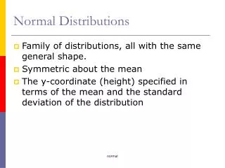
Standardizing the Data We have seen that normal curves don’t all look alike, but this is only a matter ofperception. In fact, all normal distributions tell the same underlying story but useslightly different dialects to do it. One way to understand the story of any givennormal distribution is to rephrase it in a simple common language–a languagethat uses the mean and the standard deviation as its only vocabulary. Thisprocess is called standardizing the data.
z-value To standardize a data value x, we measure how far x has strayed from themean using the standard deviation as the unit of measurement.A standardizeddata value is often referred to as a z-value. The best way to illustrate the process of standardizing normal data is bymeans of a few examples.
Example 16.4 Standardizing Normal Data Let’s consider a normally distributed data set with mean = 45ft and standarddeviation = 10 ft. We will standardize several data values, starting with a couple of easy cases.
Example 16.4 Standardizing Normal Data ■x1= 55ft is a data point located 10 ft above (A in the figure) the mean = 45 ft.
Example 16.4 Standardizing Normal Data ■Coincidentally, 10 ft happens to be exactly one standard deviation. The fact thatx1= 55ft is located one standard deviation above the meancan be rephrased by saying that the standardized valueofx1= 55 is z1= 1.
Example 16.4 Standardizing Normal Data ■x2= 35ft is a data point located 10 ft (i.e., one standard deviation) below the mean (B in the figure). This means that thestandardized valueof x2= 35 is z2= –1.
Example 16.4 Standardizing Normal Data ■x3= 50ft is a data point that is 5 ft (i.e., half a standard deviation) above the mean (C in the figure). This means that thestandardized valueof x3= 50 is z3= 0.5.
Example 16.4 Standardizing Normal Data ■x4 = 21.58 is ... uh, this is a slightly more complicated case. How do we handle this one? First, we find the signed distance between the data value andthe mean by taking their difference (x4– ). In this case we get 21.58 ft –45 ft= –23.42 ft.(Notice that for data values smaller than the mean this difference will be negative.)
Example 16.4 Standardizing Normal Data ■If we divide this difference by = 10 ft, we get the standardized valuez4= –2.342. This tells us the data point x4 is –2.342 standard deviations from the mean = 45 ft (D in the figure).
Standardizing Values In Example 16.4 we were somewhat fortunate in that the standard deviationwas = 10,an especially easy number to work with. It helped us get our feetwet. What do we do in more realistic situations, when the mean and standarddeviation may not be such nice round numbers? Other than the fact that we mayneed a calculator to do the arithmetic, the basic idea we used in Example 16.4remains the same.
STANDARDIZING RULE In a normal distribution with mean and standard deviation , the standardizedvalue of a data point x is z = (x – )/.
Example 16.5 Standardizing Normal Data: Part 2 This time we will consider a normally distributed data set with mean = 63.18 lband standard deviation = 13.27 lb. What is the standardizedvalue of x = 91.54 lb? This looks nasty, but with a calculator, it’s a piece of cake: z = (x – )/ = (91.54 – 63.18)/13.27 = 28.36/13.27 ≈ 2.14
Example 16.5 Standardizing Normal Data: Part 2 One important point to note is that while the original data is given in pounds,there are no units given for the z-value. The units for the z-value are standarddeviations, and this is implicit in the very fact that it is a z-value.
Finding the Value of a Data Point The process of standardizing data can also be reversed, and given a z-valuewe can go back and find the corresponding x-value. All we have to do is take theformulaz = (x – )/ and solve for x in terms of z. When we do this we get theequivalent formula x = + •z. Given , , and a value for z, this formula allows us to “unstandardize” z and find the original data value x.
Example 16.6 “Unstandardizing” az-Value Consider a normal distribution with mean = 235.7m and standard deviation = 41.58m. What is the data value x that corresponds to the standardized z-value z = –3.45?
Example 16.6 “Unstandardizing” az-Value We first compute the value of –3.45 standard deviations: –3.45 = –3.45 41.58 m = –143.451 m. The negative sign indicates that the data pointis to be located below the mean. Thus,x = 235.7 m – 143.451 m = 92.249 m.