Download
1 / 21
210 likes | 328 Vues
Free Energies via Velocity Estimates. B.T. Welsch & G.H. Fisher, Space Sciences Lab, UC Berkeley. In ideal MHD, photospheric flows move mag-netic flux with a flux transport rate , B n u f. (1). Demoulin & Berger (2003): Apparent motion of flux on a surface can arise from

E N D
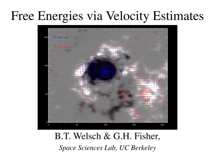
Free Energies via Velocity Estimates B.T. Welsch & G.H. Fisher, Space Sciences Lab, UC Berkeley
In ideal MHD, photospheric flows move mag-netic flux with a flux transport rate, Bnuf. (1) Demoulin & Berger (2003): Apparent motion of flux on a surface can arise from horizontal and/or vertical flows. In either case, uf represents “flux transport velocity.”
Magnetic diffusivity also causes flux transport, as field lines can slip through the plasma. • Even non-ideal transport can be represented as a flux transport velocity. • Quantitatively, one can approximate 3-D non-ideal effects as 2-D diffusion, in Fick’s Law form,
The change in the actual magnetic energy is given by the Poynting flux, c(E x B)/4. • In ideal MHD, E = -(v x B)/c, so: • uf is the flux transport velocity from eqn. (1) • uf is related to the induction eqn’s z-component, (2)
A “Poynting-like” flux can be derived for the potential magnetic field, B(P), too. • B evolves via the induction equation, meaning its connectivity is preserved (or nearly so for small ). • B(P) does not necessarily obey the induction equation, meaning its connectivity can change! • Welsch (2006) derived a “Poynting-like” flux for B(P):
The “free energy flux” (FEF) density is the difference between energy fluxes into B and B(P). (4) Depends on photospheric (Bx, By, Bz), (ux,uy), and (Bx(P), By(P)). Requires vector magnetograms. Compute from Bz. What about v or u?
Several techniques exist to determine velocities required to calculate the free energy flux density. • Time series of vector magnetograms can be used with: • FLCT, ILCT (Welsch et al. 2004), • MEF (Longcope 2004), • MSR (Georgoulis & LaBonte 2006), • DAVE (Schuck, 2006), or • LCT (e.g., Démoulin & Berger 2003) to find • Proposed locations of free energy injection can be tested, e.g., rotating sunspots & shearing along PILs.
We use ILCT to modify the FLCT flows, via the induction equation, to match Bz/t. With and the approximation uf uLCT, solving with (v·B) = 0, completely specifies (vx, vy, vz).
Tests with simulated data show that LCT underestimates Sz more than ILCT does. Images from Welsch et al., in prep.
The spatially integrated free energy flux density quantifies the flux across the magnetogram FOV. (5) • Large tU(F) > 0 could lead to flares/CMEs. • Small flares can dissipate U(F), but should not dissipate much magnetic helicity. • Hence, tracking helicity flux is important, too!
We used both LCT & ILCT to derive flows between pairs of boxcar- averaged m’grams. = 15 pix thr(|Bz|) = 100 G
Poynting fluxes into AR 8210 from ILCT & LCT both show increasing magnetic energy, U. ILCT shows an increase of ~5 x 1031 erg; FLCT shows an increase of ~1 x 1031 erg
Fluxes into the potential field, Sz(P), calculated from ILCT & FLCT flows, however, strongly disagree. Recall that Sz(F) = Sz- Sz(P), so the increase seen in ILCT’s Sz(P) will cause a decrease in Sz(F).
Changes in U(F) derived via ILCT are ~1031erg, and vary in both sign and magnitude. Changes in U(F) derived via FLCT are much smaller, and not well correlated with ILCT.
The cumulative FEFs ( U(F)) do not match; ILCT shows decreasing U(F), LCT does not.
Conclusions Re: FEF • Both FLCT & ILCT show an increase in magnetic energy U, of roughly ~1031 erg and ~5 x 1031 erg, resp. • FLCT also shows an increase in free energy U(F), of about ~1031 erg over the ~ 6 hr magnetogram sequence. • ILCT, however, shows a decrease in U(F), of ~4 x1031 erg • Apparently, this arises from a pathology in the estimation of the change in potential field energy, U(P). • This shortcoming should be easily surmountable.
References • Démoulin & Berger, 2003: Magnetic Energy and Helicity Fluxes at the Photospheric Level, Démoulin, P., and Berger, M. A. Sol. Phys., v. 215, p. 203. • Longcope, 2004:Inferring a Photospheric Velocity Field from a Sequence of Vector Magnetograms: The Minimum Energy Fit, ApJ, v. 612, p. 1181-1192. • Georgoulis & LaBonte, 2006:Reconstruction of an Inductive Velocity Field Vector from Doppler Motions and a Pair of Solar Vector Magnetograms, Georgoulis, M.K. and LaBonte, B.J., ApJ, v. 636, p 475. • Schuck, 2006:Tracking Magnetic Footpoints with the Magnetic Induction Equation, ApJv. 646, p. 1358. • Welsch et al., 2004:ILCT: Recovering Photospheric Velocities from Magnetograms by Combining the Induction Equation with Local Correlation Tracking, Welsch, B. T., Fisher, G. H., Abbett, W.P., and Regniér, S., ApJ, v. 610, p. 1148. • Welsch, 2006:Magnetic Flux Cancellation and Coronal Magnetic Energy, Welsch, B. T, ApJ, v. 638, p. 1101.
Also works w/ non-ideal terms… at eqn’s left is valid w/any non-ideal term!