Download
1 / 24
240 likes | 459 Vues
Machine vision is not a subset of:. Computer Science Image Processing Pattern Recognition Artificial Intelligence (whatever this is!) However, tools and concepts from these areas are often applied to vision applications. Machine vision is.

E N D
Machine vision is not a subset of: • Computer Science • Image Processing • Pattern Recognition • Artificial Intelligence (whatever this is!) However, tools and concepts from these areas are often applied to vision applications.
Machine vision is • “…the use of devices for optical, non-contact sensing to receive and interpret an image of a real scene automatically, in order to obtain information and or control machines or processes."Automated Vision Association, 1985
Machine vision Requires • Mechanical handling • Lighting • Optics, including conventional imaging, lasers, diffractive optics, fiber optics, etc. • Sensors (Cameras) • Electronics (analog and digital) • Digital systems architecture • Software
Illumination Invariance A Simple 1-D Model For Illumination Incident light reaching a linear sensor can be expressed as: I[n]=I0[n]s[n] In which I[n] is the light reaching the nth pixel, L[n] is the background illumination and s[n] is the value of reflection or transmission of the object being observed which can range between 0 and 1.
Video Signal Generation The sensor converts the light into an electrical signal v[n] v[n] = b[n]s[n] in which b[n] is proportional to I0[n]. • In many vision applications, b[n] varies slowly as a function of distance because background illumination does not change rapidly.
Scan Line from Hypothetical Image • Small objects have 50% contrast with background • Background illumination variations can be caused by optics and lighting • The objective here is to find the dark features!
Ideal Low-Pass Filter • Filtering provides an estimate of b[n]. • Subtracting the original image from the low-pass filtered image provides the lower curve: yhp[n] = b[n]s[n] ‑ b[n] = b[n](s[n] - 1)
Linear High-Pass Filtering • Results on previous slide show that the resulting high-pass filtering provides a significant improvement in the detection of dark features. • A single threshold can be selected which will detect all of the features but the sensitivity varies because of the illumination level. • Differentiating between features with different contrast values would be difficult, however.
Illumination-Invariant Processing • Transforming image pixel values logarithmically, however, removes the effects of varying illumination. • A logarithmic image is sometimes referred to as a density image using medical imaging concepts. • A single threshold will detect all features equally well regardless of light level.
Background Illumination • Background illumination for the following discussion refers to the source or sources that illuminate a given scene. • The illumination may be either from the front or back but not from both at the same time. • Background illumination may be measured directly in some vision applications but has to be estimated in others. • If the background can be measured directly or estimated, illumination-invariant techniques can be employed so that a feature in a scene may be extracted regardless of the illumination level at the feature’s location.
Homomorphic Filtering Inverse Nonlinear Transform • One classical image enhancement technique is based on combining linear filtering with a nonlinear point transform of the gray-scale values of the input image. • If a logarithmic transform is used, the result is illumination invariant. • The inverse operation is not useful when the results will be thresholded. Nonlinear Transform Output Image High-Pass Filter Input Image
Homomorphic example High-Pass Filtering Homomorphic Filtering Original Image Log Transformed
Linear Filtering Limitations • In the hypothetical example, an assumption was made that a linear filter could be obtained that would filter out the dark features. • In actuality, this turns out to be difficult to accomplish and implementation requires complicated (and therefor computationally intensive) algorithms and may very well not provide a good estimate of the background illumination. • As will be shown, however, it is still possible to obtain illumination-invariant results.
Illumination Invariant FIR Filter Consider a FIR filter that will remove the DC component over a neighborhood Assuming that all pixels have gray-scale value , then From this, it can be inferred that
Invariant Filter Output Now, since v[n] = s[n]b[n] For slowly varying illumination, b[k] is assumed to be the constant over the filter extent so y[n] does not depend on illumination:
Morphological Background Estimation • For an image containing dark regions smaller than some given structuring element, a gray-scale closing operation can be used to estimate the background. • With a good estimate of the background, an illumination invariant output is still obtained.
Slow and Fast Illumination Changes • Illumination changes can occur over a variety of time spans. • Slow variations are often associated with filament evaporation in incandescent lamps and similar aging effects. • Slow variations can, in some cases, be corrected by viewing a diffuse uniform reflector periodically. • Rapid variations are often associated with voltage fluctuations and ripple due to sinusoidal driving voltages.
Short-Term Compensation • Regulated DC sources can be used for the illumination sources but is quite expensive for high-power applications. • In some applications, cameras can be scanned synchronously with the power line although AC power regulation may still be required, i.e. Sola transformers. • This approach, however, is unsuitable for high-speed matrix and line-scan camera applications.
Alternative Short-Term Compensation • Suppose that the effective illumination reaching the sensor is a function of both time and spatial position: I[j,n] =I0[j,n]s[j,n] • Since illumination sources are usually driven from a common power source, the light output of each illumination source will vary temporally in exactly the same manner so that I0[j,n] can be decomposed into the product: I0[j,n] = It[j]Is[n] • The voltage output of the sensor becomes v[j,n] = It[j]b[n]s[j,n]
Short Termp Compensation (cont.) • The density representation becomes d[j,n] = log(It[j]b[n]s[j,n]) = log(It[j]) + log(b[n]s[j,n]) • Let a[j] be the average value of the N density-image pixels in a reference region which never changes for the jth sample: logIt[j] is constant for all pixels in region R since it only varies as a function of the sample number.
Short Termp Compensation (cont.) A constant kR can be defined as A normalized image in which compensation for the short-term variations are provided follows: dn[j,n] = logIt[j] + log(b[n]s[j,n] - a[j] = logIt[j] + log(b[n]s[j,n] - log(It[j]) - kR =log(b[n]s[j,n]) - kR the amount of processing required is relatively small. The region R need only be large enough to minimize errors due to camera signal noise. The image normalization operation simply requires that a constant value be added to each pixel
Quantization Considerations • Effects of quantization error when logarithmic transformation is performed before (nearly horizontal line) after (approximately triangular waveform). • The lower and higher ramps represent background and foreground data.
Accidental Illumination Invariance • Scaled gamma correction with an exponent of .45 (top curve) and logarithmic transformation function (bottom curve) are very similar except for low gray levels. • Enabling gamma correction can provide a good approximation to a logarithmic transformation. • The SNR of typical video cameras probably does not justify a better approximation
Image Format Considerations • GIF: The original Compuserve format! • JPEG: Very good compression available. • BMP: The Windows standard. • PCX: The original PC paintbrush format • TIFF: The almost universal standard ! • PGM: Portable Gray Map: No Endian Problems! • Irfan View reads all of the above and many more!