Download
1 / 14
150 likes | 343 Vues
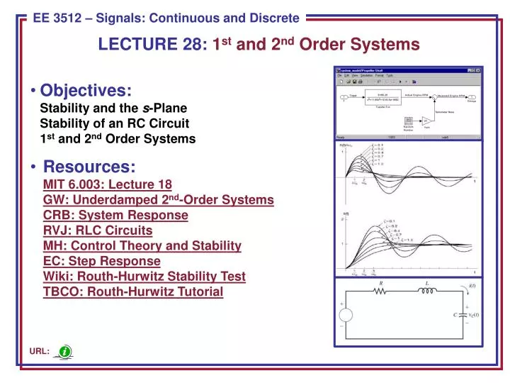
LECTURE 28: 1 st and 2 nd Order Systems. Objectives: Stability and the s -Plane Stability of an RC Circuit 1 st and 2 nd Order Systems

E N D
LECTURE 28: 1st and 2nd Order Systems • Objectives:Stability and the s-PlaneStability of an RC Circuit1st and 2nd Order Systems • Resources:MIT 6.003: Lecture 18GW: Underdamped 2nd-Order SystemsCRB: System ResponseRVJ: RLC CircuitsMH: Control Theory and StabilityEC: Step ResponseWiki: Routh-Hurwitz Stability TestTBCO: Routh-Hurwitz Tutorial URL:
Stability of CT Systems in the s-Plane • Recall our stability condition for the Laplace transform of the impulse response of a CT linear time-invariant system: • This implies the poles are in the left-half plane.This also implies: • A system is said to be marginally stableif its impulse response is bounded: • In this case, at least one pole of the systemlies on the jω-axis. • Recall periodic signals also have poles on the jω-axis because they are marginally stable. • Also recall that the left-half plane maps to the inside of the unit circle in the z-plane for discrete-time (sampled) signals. • We can show that circuits built from passive components (RLC) are always stable if there is some resistance in the circuit. LHP
Stability of CT Systems in the s-Plane • Example: Series RLC Circuit • Using the quadratic formula: The RLC circuitis always stable. Why?
Analysis of the Step Response For A 1st-Order System • Recall the transfer function for a1st-order differential equation: num = 1; den = [1 –p]; t = 0:0.05:10; y = step(num, den, t); • Define a time constant as the time it takes for the response to reach 1/e (37%) of its value. • The time constant in this case is equal to-1/p. Hence, the real part of the pole, which is the distance of the pole from the jω-axis, and is the bandwidth of the pole, is directly related to the time constant.
Second-Order Transfer Function • Recall our expression for a simple, 2nd-order differential equation: • Write this in terms of two parameters, ζand ωn, related to the poles: • From the quadratic equation: • There are three types of interestingbehavior of this system: Impulse Response Step Response
Step Response For Two Real Poles • When ζ> 1, both poles arereal and distinct: • When ζ= 1, both poles arereal (s=ωn) and repeated: • There are two componentsto this response:
Step Response For Two Real Poles (Cont.) Both Real and Repeated Two Real Poles • ζis referred to as the damping ratio because it controls the time constant of the impulse response (and the time to reach steady state); • ωnis the natural frequency and controls the frequency of oscillation (which we will see next for the case of two complex poles). • ζ> 1: The system is considered overdamped because it does not achieve oscillation and simply directly approaches its steady-state value. • ζ= 1: The system is considered critically damped because it is on the verge of oscillation.
Step Response For Two Complex Poles • When 0 < ζ< 1, we have two complex conjugate poles: • The transfer function can be rewritten as: • The step response, after some simplification, can be written as: • Hence, the response of this system eventually settles to a steady-state value of 1. However, the response can overshoot the steady-state value and will oscillate around it, eventually settling in to its final value.
Analysis of the Step Response For Two Complex Poles Impulse Response • ζ> 1: the overdamped system experiences an exponential rise and decay. Its asymptotic behavior is a decaying exponential. • ζ= 1: the critically damped system has a fast rise time, and converges to the steady-state value in an exponetial fashion. • 0 < ζ> 1: the underdamped system oscillates about the steady-state behavior at a frequency of ωd. • Note that you cannot control the rise time and the oscillation behavior independently! • What can we conclude about the frequency response of this system? Step Response
Implications in the s-Plane • Several important observations: • The pole locations are: • Since the frequencyresponse is computedalong the jω-axis, we can see that the pole islocated at ±ωd. • The bandwidth of thepole is proportional to the distance from the jω-axis, and is given by ζωn. • For a fixed ωn, the range 0 < < 1describes a circle. We will make use of this concept in the next chapter when we discuss control systems. • What happens if ζis negative?
RC Circuit • Example: Find the response to asinewave:. • Solution: • Again we see the solution is the superposition of a transient and steady-state response. • The steady-state response could have been found by simply evaluating the Fourier transform at ω0and applying the magnitude scaling and phase shift to the input signal. Why? • The Fourier transform is given by:
Summary • Reviewed stability of CT systems in terms of the location of the poles in the s-plane. • Demonstrated that an RLC circuit is unconditionally stable. • Analyzed the properties of the impulse response of a first-order differential equation. • Analyzed the behavior of stable 2nd-order systems. • Characterized these systems in terms of three possible behaviors: overdamped, critically-damped, or overdamped. • Discussed the implications of this in the time and frequency domains. • Analyzed the response of an RC circuit to a sinewave. • Next: Frequency response, Bode plots and filters.
The Routh-Hurwitz Stability Test • The procedures for determining stability do not require finding the roots of the denominator polynomial, which can be a daunting task for a high-order system (e.g., 32 poles). • The Routh-Hurwitz stability test is a method of determining stability using simple algebraic operations on the polynomial coefficients. It is best demonstrated through an example. • Consider: • Construct the Routh array: Number of sign changes in 1st column = number of poles in the RHPRLC circuit is always stable
Routh-Hurwitz Examples • Example: • Example: