Download
1 / 14
140 likes | 349 Vues
In order to solve this equation, the first item to consider is: “How many solutions are there?” Let’s look at some equations and consider the number of solutions. Equation Solution set. Number of solutions.

E N D
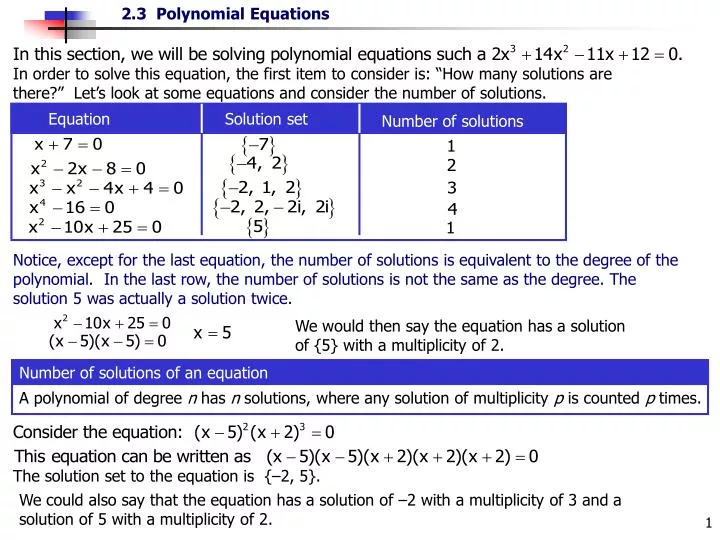
In order to solve this equation, the first item to consider is: “How many solutions are there?” Let’s look at some equations and consider the number of solutions. Equation Solution set Number of solutions We would then say the equation has a solution of {5} with a multiplicity of 2. Number of solutions of an equation A polynomial of degree n has n solutions, where any solution of multiplicity p is counted p times. Notice, except for the last equation, the number of solutions is equivalent to the degree of the polynomial. In the last row, the number of solutions is not the same as the degree. The solution 5 was actually a solution twice. The solution set to the equation is {–2, 5}. We could also say that the equation has a solution of –2 with a multiplicity of 3 and a solution of 5 with a multiplicity of 2.
Finding Rational Solutions The previous section contained factoring polynomials of degree 3 or more. This section concentrates on techniques for solving polynomials of degree 3 or more. In the previous section, one factor was given. After showing the binomial x – c was a factor, the complete factorization could be obtained by factoring the quotient. Rational Root Theorem Consider the polynomial equation In this section no factors will be given. So there will be a little trial and error. Theorems, properties and rules will be used to create a procedure for solving these types of equations. The following theorem will give a set of potential rational solutions of polynomial equations. An example of how this theorem is used is on the following slide.
Example 1. Use the rational root theorem to give all possible rational roots for the equation (do not solve): Answer: Your Turn Problem #1 Use the rational root theorem to give all possible rational roots for the equation (do not solve): The possible solutions are the combinations of Find all factors of c and d Notice the number of possible solutions that exist. There are 16 possible solutions. Since the degree of the polynomial is 4, at least 12 of these will not be a solution. Recall in the previous section, a polynomial of degree 3 or 4 was to be factored. To solve these equations, the first step is to factor and then set each factor equal to zero and solve. However in the previous section, one solution was given. We were then able to use synthetic division and complete the factorization. In this section, no solution will be given. We need to find one from the list of possible solutions. In the last Your Turn Problem, there were 16 possibilities. It is possible only two will be solutions. Finding the first solution is the most time consuming. Usually once one solution is found, the others will be easier to find.
Example 2. Use the rational root theorem and the factor theorem to help solve the equation: Solution: Once one root is found, the polynomial can be written in factored form. Your Turn Problem #2 Use the rational root theorem and the factor theorem to help solve the equation: Write a list of all possible solutions: Since we have a degree 3 polynomial, once one solution is found, the other two can be found by factoring or by using the quadratic formula. Find the first root (solution) using the possible solutions and synthetic division. This may take a few tries. Now complete the factorization and find all 3 roots.
Example 3. Use the rational root theorem and the factor theorem to help solve the equation: Solution: Your Turn Problem #3 Use the rational root theorem and the factor theorem to help solve the equation: Write a list of all possible solutions: Hopefully, one or more of the integers is a root. If not, it will be necessary to check if one of the fractions is a root. Once one root is found, the polynomial can be written in factored form. Now complete the factorization and find all 3 roots.
Once one solution is found in a 3rd degree polynomial, a trinomial is left to be factored to obtain the last two solutions. If the trinomial can not be factored, then quadratic equation must be used. Solution: Your Turn Problem #4 Use the rational root theorem and the factor theorem to help solve the equation: List all possible solutions: Once one root is found, the polynomial can be written in factored form. Since the trinomial can not be factored, use the quadratic equation to solve.
Nonreal complex solutions of polynomial equations with real coefficients, if they exist, must occur in conjugate pairs. Usually we obtain complex number solutions when we use the quadratic formula or the square root property. If the number under the square root is negative, this will give a complex number. Since there is a in front of the radical, there will be two complex number solutions. Solution: Your Turn Problem #5 Use the rational root theorem and the factor theorem to help solve the equation: List all possible solutions: Use the square root property to solve.
As you have noticed, solving these polynomial equations can be quite time consuming. You should try and convince yourself that you are having a good time so it doesn’t seem so bad. Also, a couple of rules will be introduced which can make this process not as difficult. Descartes’ Rule of Signs If P(x) is a polynomial with real coefficients: The number of positive roots of P(x)=0 is either equal to the number of variations in sign of P(x) or less than that by an even number. The number of negative roots of P(x)=0 is either equal to the number of variations in sign of P(–x) or less than that by an even number. “Less than that by an even number”: complex solutions occur in conjugate pairs. We then always subtract by multiples two because the solutions may be complex. For example; If you get 2 changes for P(x), then you answer: 2 or 0 positive solutions. If you get 3 changes for P(x), then you answer: 3 or 1 positive solutions. If you get 4 changes for P(x), then you answer: 4 or 2 or 0 positive solutions. If you get 5 changes for P(x), then you answer: 5 or 3 or 1 positive solutions. If you get 1 changes for P(x), then you answer: 1 positive solution.
Example 6. Use Descartes’ Rule of Signs to list the possibilities for the number of positive and negative solutions of the equation (do not solve): To find the number of positive solutions, count the sign changes of P(x). Your Turn Problem #6 Use Descartes’ Rule of Signs to help list the possibilities for the nature of the solutions of the equation (do not solve): There are no variations in sign of P(x), therefore there are no positive solutions. To find the number of negative solutions, replace x with –x and simplify. Then count the sign changes of P(–x). There are 3 variations in sign, therefore there are 3 or 1 negative solutions. Answer: No positive solutions, 3 or 1 negative solutions. Answer: There are 3 or 1 positive solutions. Zero negative solutions
Example 7. Use Descartes’ Rule of Signs to help list the possibilities for the nature of the solutions of the equation (do not solve): Count the number in variations of sign of the polynomial P(x). Your Turn Problem #7 Use Descartes’ Rule of Signs to help list the possibilities for the nature of the solutions of the equation (do not solve): There are 3 variations in sign, therefore there are 3 or 1 positive solutions. To find the number of negative solutions, replace x with –x and simplify. Then count the sign changes of P(–x). There is 1 variation in sign, therefore there is 1 negative solution. Answer: 3 or 1 positive solutions, 1 negative solutions. Answer: 3 or 1 positive solutions, 1 negative solutions.
Example 8. Use Descartes’ Rule of Signs to help list the possibilities for the nature of the solutions of the equation (do not solve): Count the number in variations of sign of the polynomial P(x). Your Turn Problem #8 Use Descartes’ Rule of Signs to help list the possibilities for the nature of the solutions of the equation (do not solve): There are 3 variations in sign, therefore there are 3 or 1 positive solutions. To find the number of negative solutions, replace x with –x and simplify. Then count the sign changes of P(–x). There are 2 variations in sign, therefore there are 2 or 0 negative solutions. Answer: 3 or 1 positive solutions, 2 or 0 negative solutions. Answer: 2 or 0 positive solutions, 3 or 1 negative solutions.
This rule only gives us information about the possible solutions. Let’s see how this information can make the process easier. Solution: Using the quadratic formula to solve. Your Turn Problem #9 Hint: Should you try positive numbers? Descartes’ Rule tells us that there are 3 or 1 positive solutions and no negative solutions (verify). This just cut or list from 8 possible solutions to 4 possible solutions. Therefore do not try any negative numbers using synthetic division.
All of the previous examples and your turn problems contained 3rd degree polynomials. Once one solution is found, the other two can be found by factoring or by using the quadratic formula. If the equation to be solved is a 4th degree polynomial, once one solution is found, the factor obtained will be a 3rd degree polynomial (often called the depressed polynomial). Since we still have a 3rd degree polynomial, we still need to find another solution to obtain a depressed polynomial of degree 2. So if we have a 4th degree polynomial, we will need to find 2 solutions by synthetic division to obtain a depressed polynomial of degree 2. If we have a 5th degree polynomial, 3 solutions will need to found using synthetic division to obtain a depressed polynomial of degree 2. In general, the number of solutions needed to found using synthetic division will always be two less than the degree of the equation to solved. The next example will show this concept. Next Slide
Solution: Your Turn Problem #10 Find one solution using synthetic division. Once one solution is found, find another solution using synthetic division. However, when finding the second, use the depressed polynomial found by finding the first solution. (Hint start with c = -1) Once one root is found, the polynomial can be written in factored form. However, the depressed polynomial is of degree 3. Therefore we need to find a second solution to obtain a depressed polynomial of degree 2. (Hint: use c= 2) Now we can write the equation in factored form and obtain the 4 solutions. The End. B.R. 2-26-07