Download
1 / 27
270 likes | 380 Vues
Table 8.11. Table 8.1. Table 8.2. Note: There are (# of Treatment Combinations)! number of possible ways to test these factors and levels (“Run Combinations”). Pick one randomly to do your testing. Don’t always test in a pre-described order. Table 8.3. Table 8.4. Figure 8.2. Eq. 1.

E N D
Table 8.2 Note: There are (# of Treatment Combinations)! number of possible ways to test these factors and levels (“Run Combinations”). Pick one randomly to do your testing. Don’t always test in a pre-described order.
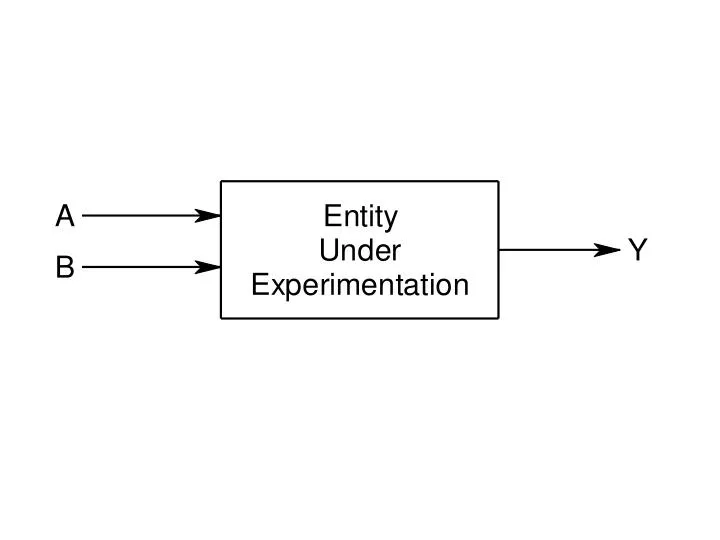
Eq. 1 “A main effect” The “A main effect” is the average change in Y when factor A changes from low to high (- to +) A is the average change from the bottom to the top of the square.
Eq. 2 “B main effect” The “B main effect” is the average change in Y when factor B changes from low to high (- to +) B is the average change from the left to the right side of the square.
Eq. 3 AB is the difference in the average of the responses across both diagonals of the square. AB is a measure of the interaction between factors A and B.
Eq. 4 Eq. 5
Table 8.7 Table 8.8
kI = ((1)+b+a+ab)/4 Eq. 6a kA = (-(1)-b+a+ab)/4 Eq. 6b kB = (-(1)+b-a+ab)/4 Eq. 6c kAB = ((1)-b-a+ab)/4 Eq. 6d Y = kI+kAXA+ kBXB+ kABXAXB Eq. 7
Example: RC Circuit Example: RC Circuit
Tables 8.7 and 8.8 Example: RC Circuit
km = ((1)+b+a+ab)/4 Eq. 6a kA = (-(1)-b+a+ab)/4 Eq. 6b kB = (-(1)+b-a+ab)/4 Eq. 6c kAB = ((1)-b-a+ab)/4 Eq. 6d Y = km+kAXA+ kBXB+ kABXAXB Eq. 7 km = ((1)+b+a+ab)/4 = (350+420+360+440)/4 = 392.5 msec. kA = (-(1)-b+a+ab)/4 = (-350-420+360+440)/4 = 7.5 msec. kB = (-(1)+b-a+ab)/4 = (-350+420-360+440)/4 = 37.5 msec. kAB = ((1)-b-a+ab)/4 = (1570+30+150+10)/4 = 2.5 msec. t = 392.5 + 7.5XA+ 37.5XB+ 2.5XAXB msec.
Table 8.9 km = ((1)+b+a+ab)/12 Eq. 8a kA = (-(1)-b+a+ab)/12 Eq. 8b kB = (-(1)+b-a+ab)/12 Eq. 8c kAB = ((1)-b-a+ab)/12 Eq. 8d
km = ((1)+c+b+bc+a+ac+ab+abc))/8m Eq. 9a kA = (-(1)-c-b-bc+a+ac+ab+abc))/8m Eq. 9b kB =(-(1)-c+b+bc-a-ac+ab+abc))/8m Eq. 9c kC =(-(1)+c-b+bc-a+ac-ab+abc))/8m Eq. 9d kAB =((1)+c-b-bc-a-ac+ab+abc))/8m Eq. 9e kAC =((1)-c+b-bc-a+ac-ab+abc))/8m Eq. 9f kBC =((1)-c-b+bc+a-ac-ab+abc))/8m Eq. 9g kABC = (-(1)+c+b-bc+a-ac-ab+abc))/8m Eq. 9h Y = km+ kAXA+ kBXB+ kCXC+ kABXAXB + kACXAXC+ kBCXBXC+kABCXAXBXCEq. 10