Download
1 / 46
460 likes | 574 Vues
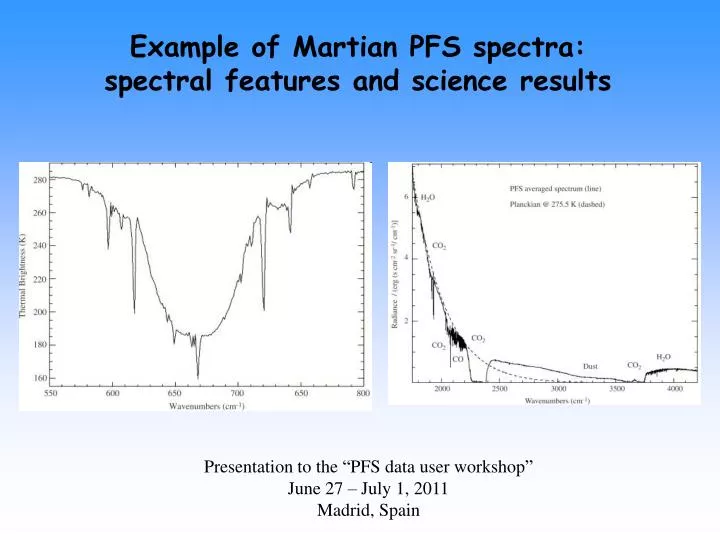
Example of Martian PFS spectra: spectral features and science results. Presentation to the “PFS data user workshop” June 27 – July 1, 2011 Madrid, Spain.

E N D
Example of Martian PFS spectra: spectral features and science results Presentation to the “PFS data user workshop” June 27 – July 1, 2011 Madrid, Spain
Single spectra measured by PFS south of the Volcano (gray), on top the caldera (top) and north of it in the plain (bottom). Only a short part of the SW channel spectrum is shown, to evidence the decrease of the CO2 and CO on top of the mountain. Giuranna et al., 2005, ‘Calibration of the Planetary Fourier Spectrometer short Wavelenghth channel’, Planetary and Space Science 53, pp. 975-991
The CO absorption lines in the 4.7 μm range. The synthetic spectrum is computed for 825 ppm of CO and is shown shifted by 0.45 CGS units for comparison. Simulation of the = 1-0 band of carbon monoxide.
Observations of CO in the atmosphere of Mars with PFS Billebaud et al. (2009) - PSS 57, 1446–1457 G. Sindoni et al, 2011, PSS59, 149-162
Observations of CO in the atmosphere of Mars with PFS onboard Mars Express Data fromLs=331° (MY26) to Ls=51.61°(MY27) have been analyzed. Set of spectra fitted with synthetic spectra. The corresponding retrieved CO mixing ratios are (from left to right and top to bottom): 7.5×10⁻⁴, 9.3×10⁻⁴, 8.7×10⁻⁴, and 9.7×10⁻⁴. Billebaud et al., 2009, ‘Observations of CO in the atmosphere of Mars with PFS onboard Mars Express’, Planetary and Space Science 57, pp. 1446-1457
Observations of CO in the atmosphere of Mars with PFS onboard Mars Express Surface pressure (coming from the MCD model) as a function of latitude for three LS ranges. From left to right and top to bottom: (a) 331–360°, (b) 0–30°, and (c) 30–52° The other parameters are mixed. CO mixing ratios retrieved as a function of surface pressure for three latitude ranges. Upper left: less than -30° . Upper right: between -30° and 30°. Bottom: higher than 30°. The other parameters are mixed.
Observations of water vapour and carbon monoxide in the Martian atmosphere with the SWC of PFS/MEX Examples of continuum definition for PFS measured spectra in the absorption band spectral ranges for the CO. The black line is the measured spectrum and the red line is its continuum. The crosses are the spectral point used for the continuum definition. Spectral fit example of the carbon monoxide absorption band. Data set from Ls=62° (MY27) to Ls=203° (MY29). Sindoni et al., 2011, ‘Observations of water vapour and carbon monoxide in the Martian atmosphere with the SWC of PFS/MEX’, Planetary and Space Science 59, pp. 149-162
Observations of water vapour and carbon monoxide in the Martian atmosphere with the SWC of PFS/MEX Map of retrieved concentration of carbon monoxide as a function of Longitude and Latitude as observed by PFS/SWC, from orbit 634 to orbit 6537, obtained using averaged spectra in square bins of 10° Longitude×10° Latitude for each season: Ls=0–90° (northern Spring), Ls=90−180° (northern Summer), Ls=180−270° (northern Fall) and Ls=305–360° (northern Winter). Examples of mean latitudinal trends retrieved between Ls=90° and 120° (early northern summer) (left) and between Ls=240° and 270° (late northern fall) (right).
Water lines in the 2.7 μm range. The synthetic spectrum is computed for 300 ppm of H2O and is shown shifted by 0.5 CGS units for a better comparison.
Investigation of water vapor on Mars with PFS/SW of Mars Express The seasonal map of water vapor between LS = 330◦ of MY 26 and LS = 200◦ of MY 27. The martian H2O cycle is well covered in this period and shows a clear summer maximum (the highest value is 68 pr. μm). The normalized PFS spectrum (black line), that is created from the observational spectra 61–75 of orbit 278, is fitted by the synthetic spectrum (gray line). For the H2O fitting the region between 3820 and 3900 cm−1 was used yielding a mixing ratio of 225 ppm corresponding to a column density of 19.0 pr. μm at a saturation level of 19 km above the surface. Tschimmel et al., 2008, ‘Investigation of water vapor on Mars with PFS/SW of Mars Express’, Icarus 195, pp. 557 - 575
Investigation of water vapor on Mars with PFS/SW of Mars Express For the three latitude bands of 60–90° N (upper panel), 30–60° N (middle panel) and 0–30° N (lower panel) the retrieved column densities were binned within 5° of Ls and multiplied with the respective area to get the total amount of water contained in the atmosphere of that latitude (given in 1014 g). The water vapor from the sublimation is transported by circulation further poleward and redeposited on the cold permanent ice cap. Later during the peak of the summer also this ice sublimes and produces the observed H2O peak with approximately 60 pr. m (Montmessin et al., 2004).
Investigation of water vapor on Mars with PFS/SW of Mars Express Arabia Terra Tharsis The spatial distribution of water vapor for LS = 135–200◦ (northern autumn). The column densities, normalized to 6.1 mbar, are displayed up to 30 pr. μm.
Observations of water vapour and carbon monoxide in the Martian atmosphere with the SWC of PFS/MEX Examples of continuum definition for PFS measured spectra in the absorption band spectral ranges for the H2O. The black line is the measured spectrum and the red line is its continuum. The crosses are the spectral point used for the continuum definition. Spectral fit example of the water vapour absorption bands. Data set from Ls=62° (MY27) to Ls=203° (MY29). Sindoni et al., 2011, ‘Observations of water vapour and carbon monoxide in the Martian atmosphere with the SWC of PFS/MEX’, Planetary and Space Science 59, pp. 149-162
Observations of water vapour and carbon monoxide in the Martian atmosphere with the SWC of PFS/MEX Map of retrieved abundance of water vapour as a function of Solar Longitude (Ls) and Latitude as observed by PFS/SWC, from orbit 634 to orbit 6537, obtained using spectra averaged in 5° Ls×5° Latitude bins.
PFS measured and synthetic (shifted by 1.5 CGS units) spectrum in the 6850-7700 cm−1 range showing a nonsaturated CO2 band, a few solar and many water lines. Mars spectrum as measured by PFS (bottom) together with a pure solar spectrum (top).
A solar spectrum for PFS data analysis The solar spectrum valid for PFS A portion of PFS Mars spectrum on Mars (average over 1680 measurements; orbits from 10 to 72) in which solar lines have been identified. Unknown is referred to features of uncertain origin. The broad band after 6860 cm-1 is due to atmospheric CO2. Fiorenza and Formisano, 2005, ‘A solar spectrum for PFS data analysis’, Planetary and Space Science 53, pp. 1009-1016
Planetary Fourier Spectrometer observation of CO2 (628) isotopologue on Mars Average observed spectrum (black) and the synthetic spectrum (red) computed taking the albedo constant. The modified albedo. Geminale and Formisano, 2009, ‘Planetary Fourier Spectrometer observation of CO2 (628) isotopologue on Mars’, Journal of Geophysical Research, Volume 114, Issue E2
Planetary Fourier Spectrometer observation of CO2 (628) isotopologue on Mars CO2(628) Observed spectrum (black) and synthetic spectrum (red).The isotopic ratios for CO2 (628) and CO2 (627) are 0.80 and 0.96 of terrestrial standard value, respectively. Best fit to the observed PFS average spectrum (black)
Detection of Methane in the Atmosphere of Mars Geographical distribution of the orbits considered: red (high methane mixing ratio), yellow (medium methane mixing ratio), and blue (low methane mixing ratio). Strong fluctuations occur in each of the three categories, indicating the possible presence of localized sources. Spectra with 35 ppbv of methane. The error on the measurements is shown as ±1σ confidence lines. Formisano et al., 2004, ‘Detection of Methane in the Atmosphere of Mars’, Science, Volume 306, Issue 5702, pp. 1758-1761
Mapping methane in Martian atmosphere with PFS-MEX data Average of 8249 spectra in the latitude range [30°, 50°] and all longitudes during northern fall For weak lines the equivalent width is linearly proportional to the column density: Sq are the Hitran line intensities in the range [3017.3, 3019.3] cm-1. Geminale et al., 2011, ‘Mapping methane in Martian atmosphere with PFS-MEX data’, Planetary and Space Science 59, pp. 137 - 148
Mapping methane in Martian atmosphere with PFS-MEX data Spring: Ls=[0°:90°] Summer: Ls=[90°:180°] Methane maps for each season. Methane, being a non condensable gas, has an atmospheric abundance dominated by the polar CO2 condensation in local winter. Even if we do not cover the polar regions in local winter, we can observe the increase of methane northward or southward the equator. Fall: Ls=[180°:270°] Winter: Ls=[270°:360°]
Methane source… • Internal, such as volcanoes: for 10 ppbv of CH4 one should expect 1 – 10 ppmv of SO2 • Exogenous, such as meteorites, comets or interplanetary dust particles: the amount of • methane delivered to Mars by the comets would be on the order of 1 ton yr-1 • Internal, such as a hydrogeochemical process involving serpentinization: hydration of • ultramafic silicates (Mg, Fe-rich) results first in the formation of serpentine and • molecular hydrogen. The H2 react with carbon grains or CO2 of the crustal • rocks/pores to produce methane • Biological: microbial colonies could exist in the subpermafrost aquifer environment on • Mars, where microorganisms utilize CO and/or H2, and produce methane in turn. If • microorganism existed on Mars only in the past and produced methane, that methane • could have been stored in methane-hydrates for later release. • …and sinks • UV photolysis in the middle and upper atmosphere • Oxidation by O(1D) and OH • Oxidation by H2O2 Atreya et al., 2007, ‘Methane and related trace species on Mars: Origin, loss, implications for life, and habitability’, Planetary and Space Science 55, pp. 358 - 369
Albedo and photometric study of Mars with the Planetary Fourier Spectrometer on-board the Mars Express mission The Lambert’s law: R= (ES/π)*AL *cos i Which gives for Mars: AL =RMD2/[(ES/π) cos i] where ES and RM are solar irradiance at 1 AU and Mars radiance, respectively, both at 3900 cm−1 and D is the Sun–Mars distance. With the present study, the authors intend to extract and analyze albedo properties at 7030 cm−1, where the thermal component of Mars radiance is negligible and there are no relevant features due to gas or aerosol. At this wavenumber radiance depends mainly on surface and atmospheric aerosol scattering properties. The same study has been repeated at 3900 cm−1 for comparison Esposito et al., 2007, ‘Albedo and photometric study of Mars with the Planetary Fourier Spectrometer on-board the Mars Express mission’, Icarus 186, pp. 527 - 546
Albedo and photometric study of Mars with the Planetary Fourier Spectrometer on-board the Mars Express mission Lambert albedo maps. The top panel has been extracted from the full resolved albedo map acquired by TES at a resolution of 8° per pixel by considering only the pixels corresponding to geographical points observed by PFS. The PFS Lambert map at 7030 cm−1 is in the bottom panel.
Exercise on albedo Orbit 5639: save the spectrum with scet = 159642475.28 sel_x_axes=x_axes(*,where(hk_struct.SCET_OBSERVATION_TIME eq 159642475.28)) sel_MarsRadiance=MarsRadiance(*,where(hk_struct.SCET_OBSERVATION_TIME eq 159642475.28)) save, sel_x_axes, sel_MarsRadiance,filename='orbita_5639_scet_159642475.28.sav', /verbose Save geometry information: sel_INCIDENC_EANGLE=geo_struc(where(float(geo_struc.SCET) eq float(159642475.28))).INCIDENC_EANGLE sel_SOLAR_DISTANCE=geo_struc(where(float(geo_struc.SCET) eq float(159642475.28))).SOLAR_DISTANCE save, sel_INCIDENC_EANGLE, sel_SOLAR_DISTANCE,filename='info_geo_orbit_5639_scet_159642475.28.sav', /verbose The same for orbit: 6493 scet = 180692913.09 5458 scet = 155183341.62
Analysis of CO2 non-LTE emissions at 4.3 m in the Martian atmosphere as observed by PFS/Mars Express and SWS/ISO Nadir spectra in the 4.3 m region in Mars measured by PFS. Lopez-Valverde et al., 2005, ‘Analysis of CO2 non-LTE emissions at 4,3 m in the Martian atmosphere as observed by PFS/Mars Express and SWS/ISO’, Planetary and Space Science 53, pp. 1079 - 1087
Analysis of CO2 non-LTE emissions at 4,3 m in the Martian atmosphere as observed by PFS/Mars Express and SWS/ISO Nadir spectra in the 4.3 m region in Mars measured by ISO and PFS, together with a simulation computed with the nominal non-LTE model. Nominal results but locating the observer at various altitudes within the atmosphere, from 60 to 180 km, as indicated.
Geometry of limb observations Geometry of the observations for orbit 1234, northern latitudes are given for the 71 measurements taken in this pass. Local time is 11:30. The subsolar point was at 16.3◦ N latitude.
Observations of non-LTE emission at 4–5 microns with the planetary Fourier spectrometer abord the Mars Express mission Average spectrum over the entire set of measurements. Note the presence of the CO emission at 2100 cm−1. The red line is the deep space signal, while the blue curve is a Planckian at 190 K. Formisano et al., 2006, ‘Observations of non-LTE emission at 4–5 microns with the planetary Fourier spectrometer abord the Mars Express mission’, Icarus 182, pp. 51 - 67
CO2 non-LTE emission at 4.3 mm M. Giuranna et al., in preparation 626 main isotope New isotopic bands (1st identification on Mars) FH 636 isotopic SHa + SHb FB SHa + SHb • CO2 and CO Non-LTE emission has been observed with PFS LIMB observations • Unprecedented coverage and spectral resolution • Contributions from individual bands have been identified • Emission from CO2isotopic molecules have been observed • C12/C13 isotopic ratiocan be measured from observations of Non-LTE! • Search for carbon isotopologues would help to test if life exists on Mars.
Exercise: ‘Visualize_spectrum.pro’ Select Spectrum from file ‘O2.sav’
Study of the oxygen day-glow in the Martian atmosphere with nadir data of PFS-MeX The photo-dissociation of ozone (O3) by solar UV produces molecular oxygen in an excited state: O3 + h O2(a1Δg) + O The O2(a1Δg) may be de-excited by collisions (with CO2 molecules) or emitting radiation at 1.27m. The maximum oxygen emission occurs at equinoxes over the polar regions. An emission at middle-low latitudes is observed at the aphelion with lower values respect to the polar regions. Photo-dissociation of water….. H2O + h H + OH H + O2 + CO2 HO2 + CO2 Ozone and water vapour are anti-correlated. Geminale et al., in preparation.
Study of the oxygen day-glow in the Martian atmosphere with nadir data of PFS-MeX The main emission peak is at 7882 cm-1 and at the PFS resolution many lines of the R branch (transitions with J’=J”+1) can be resolved. This allows us to retrieve the oxygen rotational temperature by means of the linear relation between the logarithm of the line intensity divided by the line strength factor and the energy of the upper rotational state. Synthetic spectra
PFS/MEX observations of the condensing CO2 south polar cap of Mars • Mosaic of Mars Express OMEGA images showing the residual south polar cap (Ls=330°–360°). It appears clearly asymmetric, the cap center being displaced by 3° far from the geographic pole. • An example of PFS-data fit used to retrieve the RSPC composition. Black: PFS SWC spectrum of the RSPC (86° S, 20° W; Ls=338°). Red: Bi-Directional Reflectance model (DISORT; Stamnes et al., 1988). Intimate granular mixture of CO2 ice, water ice and dust. Hansen et al., 2005, ‘PFS-MEX observation of ices in the residual south polar cap of Mars’, Planetary and Space Sciece 53, pp. 1089 - 1095 Giuranna et al., 2008, ‘PFS/MEX observations of the condensing CO2 south polar cap of Mars’, Icarus 197, pp. 386 - 402
PFS/MEX observations of the condensing CO2 south polar cap of Mars Spectrum with CO2 ice features vs a spectrum without ice features
Spatial variability, composition and thickness of the seasonal north polar cap of Mars in mid-spring Best-fit of region I PFS averaged spectrum. The blue curve is the spectrum measured by PFS; the black curve is a BDR model of an intimate admixture of H2O ice (20-mm) and 0.15 wt % of dust. 3D surface plot of the Martian north polar cap at Ls 40° (MEX orbit 452). The RGB colors have been obtained from the spectra in the visible range acquired by OMEGA. The altimetry is retrieved from MOLA data. Fresnel peak Best-fit of region II PFS averaged spectrum. The cyan curve is the spectrum measured by PFS; the BDR model (black curve) is a spatial mixture of 30% CO2 ice (5mm grain size) and 70% of the same water ice as in region I. The CO2 ice, in turn, is intimately mixed with 0.006wt% ofH2O ice. No dust is present in the mixture. Giuranna et al., 2007, ‘Spatial variability, composition and thickness of the seasonal north polar cap of Mars in mid-spring’, Planetary and Space Science 55, pp. 1328 - 1345
Spatial variability, composition and thickness of the seasonal north polar cap of Mars in mid-spring Best-fit of region III PFS averaged spectrum. The red curve is the spectrum measured by PFS; the BDR model (black curve) is a mixture of CO2 ice, with 0.003wt% of water ice 0.23wt% of dust. Best-fit of region IV PFS averaged spectrum. The orange curve is the spectrum measured by PFS which is best fitted by a mixture of CO2 ice (grain size is 3 mm) and 0.02wt% of dust. Water ice is present as 0.0018 wt% in the intimate mixture, and as a 50% spatial fraction with the same composition as in region I. Best-fit of region V PFS averaged spectrum. The light blue curve is the spectrum measured by PFS; the black curve is a BDR model of an intimate admixture of 5mm sized CO2 ice and 0.003wt% of water ice. No dust is required.
Exercise: ‘exercise_temperature.pro’ Select Spectrum from file ‘Mean_Spectrum_out_Olympus.sav’
Water clouds and dust aerosols observations with PFS MEX at Mars Examples of measured spectra: spectrum above Olympus Mons and spectrum in Hellas region. Surface altitude corresponding to the centers of the FOV along orbit 37. Along x-axis is the spectrum number. Numbers along the curve indicate the mean particle size in the water ice clouds, which gives the best fit of the measured spectrum. The error of the mean particle size may exceed 0.5 μm = 0 exp(-h/H0) Zasova et al., 2005, ‘Water clouds and dust aerosols observations with PFS MEX at Mars’, Planetary and Space Science 53, pp. 1065 - 1077
Tentative detection of hydrogen peroxide (H2O2) in the Martian atmosphere with Planetary Fourier Spectrometer onboard Mars Express (a) PFS averaged spectrum. H2O2 is identified at 362 cm-1 and 379 cm-1. There are two water vapor lines at 370 cm-1 and 375 cm-1. (b) The best-fit synthetic spectrum without H2O2. (c) The best-fit synthetic spectrum with H2O2 mixing ratio of 45 ppb. (d) the continuum slope (thick dotted line) and synthetic spectra (thick dashed curves) with the H2O2 mixing ratio of 0, 30, 60, 90, 120 and 150 ppb. The continuum slope would be due to emissivity of the surface. The seasonal variation of H2O2 mixing ratio was 0 - 120 ppb during the observational period from the Mars Year (MY) 27 to the MY 29. Aoki et al., 2011, ‘Tentative detection of hydrogen peroxide (H2O2) in the Martian atmosphere with Planetary Fourier Spectrometer onboard Mars Express’, in preparation.
Martian water vapor: Mars Express PFS/LW observations Example of fits of PFS spectra in the region of H2O rotational lines and CO2ν2 band. Examples are chosen to illustrate two very different seasonal and surface temperature conditions. Seasonal distribution of water. Fouchet et al., 2007, ‘Martian water vapor: Mars Express PFS/LW observations’, Icarus 190, pp. 32 - 49
Martian water vapor: Mars Express PFS/LW observations Comparison of water columns retrieved from PFS/LW and TES for measurements in common epoch. Left panel: original TES retrievals. Right panel:corrected TES retrievals, using the new version of the TES database. Geographical distribution of water. Water columns are here normalized to a common 610 Pa pressure. Top left: entire dataset. Top right: Ls=330°–60°. Bottom left: Ls=90°–150°. Bottom right: Ls=155°–210°.
CO2 isotopologues as seen with the PFS resolution in the LWC Isotopic Abundances Used for HITRAN
Conclusions • PFS has been able to study: • Minor species: CO, H2O, CH4 (geographical and seasonal distribution) • H2O2 (seasonal distribution) • CO2 (628) • O2 (seasonal distribution) • CO2 non-LTE emission • Polar caps: composition and properties • Water clouds and aerosols • More can be done: • Aerosols properties (size distributions, optical properties, chemical composition • of dust and ice clouds) • Dust: composition, properties • Other minor species • Isotopologues: HDO, 13C 16O2 , 12C16O18O for to estimate isotopic ratios • Clouds: optical properties of the atmospheric dust and ice clouds • Soil: thermal inertia, distribution of various materials, surface-atmosphere • exchange processes.