Download
1 / 29
360 likes | 586 Vues
p 0. p. p 0. p. V. V. Airspeed Measurement. The Pitot-Static system is the standard device for airspeed measurement At low speeds, this system makes use of Bernoulli’s equation to obtain V from pressures and density. Airspeed Measurement (continued).

E N D
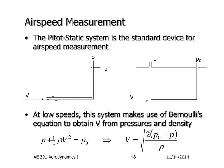
p0 p p0 p V V Airspeed Measurement • The Pitot-Static system is the standard device for airspeed measurement • At low speeds, this system makes use of Bernoulli’s equation to obtain V from pressures and density AE 301 Aerodynamics I
Airspeed Measurement (continued) • To measure the aircraft’s True Airspeed, TAS, at incompressible velocities: • However, there is no simple device for measuring density. Thus, airplane instruments are calibrated assuming sea level density, rs. • The resulting velocity is called the Equivalent Airspeed, EAS, AE 301 Aerodynamics I
Airspeed Measurement (continued) • Notice that EAS and TAS are related by the density ratio, s, • In fact, EAS is more useful to pilots since equivalent stall speed, Ve stall, is independent of altitude while true stall speed, Vtrue stall, is not!! • This is because aerodynamic forces are proportional to dynamic pressure not velocity. At the same Ve you have the same q, at any altitude! AE 301 Aerodynamics I
Airspeed Measurement (continued) • At subsonic compressible velocities, the true airspeed can be deduced from the isentropic Mach relation: • Thus, the true velocity can be found from: • The terms were rearranged since a Pitot-static system measure pressure differences! AE 301 Aerodynamics I
Airspeed Measurement (continued) • In application, aircraft instruments are calibrated assuming sea level speed of sound and pressure, as and ps. Thus, the Calibrated Airspeed, CAS, is: • Believe it or not, this relation reduces to our EAS relation at low velocities. (Homework?) • Thus CAS also has the benefit of providing a stall speed which is independent of altitude AE 301 Aerodynamics I
Airspeed Measurement (continued) • At supersonic speeds, the Pitot system is complicated by the presence of a shock wave in front of the tube. • Since the shock is non-isentropic, the total pressure being measured is less than p0. The equation accounting for this is the Rayleigh Pitot tube formula: • This relation can be used to calibrate a Mach meter p0 p02 AE 301 Aerodynamics I
Airspeed Measurement (continued) • One final note: It has been assumed thus far that the Pitot-static system correctly reads both the total and static pressure. • In practice, this is not always true. As a result, even after calibration, there may be sensor position errors in the measure airspeed. • Thus, the Indicated Airspeed, IAS, which is displayed on the cockpit instrument may differ from both EAS and CAS. AE 301 Aerodynamics I
Intro. To Viscous Flow • A lot can be learned about airplane and airfoil behavior by assuming inviscid flow. • However, most of these studies are qualified by terms like “at cruise condition”, “a well designed airfoil”, or “at moderate conditions”. • The reason is that the basic art of aerodynamic tailoring or “streamlining” is the control of undesirable viscous effects! • Thus, to understand modern aerodynamic shapes we must learn about the viscous behavior which contributed to their development. AE 301 Aerodynamics I
Viscosity • We have already described viscosity as the property of the fluid which resists shearing motion. • This property is the by-product of the random molecular motion of the particles and their ability to transport momentum. • Because gaseous viscosity is due to random particle motion, the faster the motion the greater the viscosity! I.e. viscosity increases with temperature in gasses!! • This behavior is opposite what you know about liquids - can you explain the difference? AE 301 Aerodynamics I
Viscosity (continued) • At sea level standard conditions, the value of viscosity is: • A useful equation to obtain viscosity at other temperatures is Sutherland’s formula: • where, for air, AE 301 Aerodynamics I
Reynold’s Number • A factor governing the development of viscous flow is the Reynold’s number, Re • Qualitatively, Re is a ratio of the flow momentum to the viscous force trying to retard it. • Thus, the higher the value of Re, the smaller the effect of viscosity, or visa versa • Note the subscript! The Reynold’s number depends upon a reference dimension which is specified as a subscript to avoid confusion! AE 301 Aerodynamics I
Reynold’s Number (continued) • Typical Reynold’s Number Ranges Re < 200 Plankton, protazoa, etc 200 < Re < 200 k Insects, birds 200 k < Re < 2 M UAV’s, gliders, model planes 2 M < Re < 20 M General aviation 20 M < Re < 200 M Large/high speed aircraft Re > 200 M Submarines AE 301 Aerodynamics I
Boundary Layers • Fortunately, on airfoils, viscous effects are normally restricted to a thin region near the surface - this region is called the Boundary Layer. • This fact allows us to computationally split the flow into two regions: an inviscid outer flow and a viscous near wall one. • The boundary layer has the effect of pushing flow streamlines away from the surface and thus slightly changing the effective body shape. Inviscid flow viscous flow AE 301 Aerodynamics I
Boundary Layers (continued) • Since boundary layers are thin, the pressure variation through them, normal to the surface, is very small and usually neglected. • Behind the body, the surface boundary layers merge and continue downstream as a wake. • Unlike B.L.’s, wakes are not driven by a surface shearing stress. Instead, they have a fixed amount of energy and momentum and therefor develop differently. AE 301 Aerodynamics I
Laminar flow Turbulent flow Transition Boundary Layer Development • The simpliest model of a boundary layer is that which develops over a flat plate with a sharp leading edge • There are 3 basic boundary layer regions: laminar flow, turbulent flow, and a transition region connecting them. • The laminar flow region is characterized by a smooth, steady flow similar to the inviscid flow. Only by looking at the velocity profile normal to surface is the effect of viscosity seen: x AE 301 Aerodynamics I
y d V B.L. Development (continued) • Typical laminar B.L. profile • The height above the surface where the velocity reaches 99% of the inviscid flow is called the B.L. thickness, d. • The wall shearing stress, tw, is proportional to the velocity gradient • Thus, the laminar shearing stress is the greatest at the leading edge and decreases moving downstream y x large d x small d V AE 301 Aerodynamics I
B.L. Development (continued) • As a laminar B.L. becomes thicker, it tends to become unstable. • Eventually, flow instabilities become so large that the smooth flow pattern collapses into a chaotic mixing of the fluid within the B.L. called turbulence. • The process of going from smooth laminar flow to chaotic turbulent flow is called transition. • Transition is influenced by many factors including local Reynolds number, surface roughness, freestream turbulence, etc., which make the exact transition location very difficult to predict! AE 301 Aerodynamics I
y d V laminar turbulent B.L. Development (continued) • Turbulent B.L.’s are characterized by chaotic, unsteady flow often depicted by eddies. • Turbulent flow is unsteady, but a well defined B.L. profile still exists if we consider the time average of the velocity. • A typical turbulent B.L. profile is “fuller” than a laminar one • The turbulent wall shear stress is larger than a comparable laminar one but also decreases with x. AE 301 Aerodynamics I
Shear Stress, tw Laminar flow Turbulent flow Transition B.L. Development (continued) • From the previous discussion, we can sketch the following shear stress development • Part of the drag force acting on an airfoil is found by integrating this stress. The other portion is found from the pressure forces on a body. AE 301 Aerodynamics I
Laminar Flow • For laminar flow over a flat plate a numerical solution exists if a number of assumptions are made - but the results agree very well with experiment! • The results of this solution show that a flat plate laminar B.L. grows at the rate: • where x is the distance from the leading edge. • Note how d will be thicker in more viscous fluids but thinner in flows with more momentum. AE 301 Aerodynamics I
Laminar Flow (continued) • The coefficient of friction, cf, is a non-dimension form of the wall shear stress, tw. Under this theory, the friction coefficient varies by: • And, the average friction coefficient over the length of the laminar region is: • Note that the total shearing force due to laminar flow is: AE 301 Aerodynamics I
Turbulent Laminar Turbulent Flow • Exact solutions for turbulent flow are not available, however, empirical relations based upon both theory and experiment exist. • For a flat plate with turbulent flow from the leading edge, the flat plate boundary layer thickness varies by: • Note how a turbulent boundary layer is thicker than a comparable laminar one would be since: AE 301 Aerodynamics I
Turbulent Flow (continued) • Also, the average friction coefficient over a flat plate with all turbulent flow is: • The problem with these relations is that they assume turbulent flow from the leading edge. In fact, almost all flows begin laminar and transitions to turbulent. • A little later we will see how we can use this relation for the more general case of mixed laminar and turbulent flow. AE 301 Aerodynamics I
Transition • Predicting the onset of laminar flow instability is very difficult, but do-able. • Unfortunately, the point of instability is not necessarily the critical, transition point, xcr, which generally occurs somewhere further downstream. • Instead, we must again rely upon experiment. For a flat plate, transition occurs at critical Re’s of: • The wide range in Recr is due to the different surface smoothness and freestream disturbances in the experiments. In general, Recr must be specified!! AE 301 Aerodynamics I
Friction Drag Estimation • To calculate the drag due to skin friction, first consider the case of only laminar flow: • When there is laminar flow transitioning to turbulent flow, an accurate approximation is to: • add the force due to laminar flow up to xcr • add the force as if the surface was entirely turbulent • subtract out the false turbulent contribution from the laminar region AE 301 Aerodynamics I
Pressure Gradients • The previous discussions and equations are only strictly valid for flat plates where there is no pressure gradient, dp/dx = 0. • A favorable pressure gradient is one where the pressure decreases with distance downstream, dp/dx < 0. (or dV/dx > 0!) • A favorable pressure gradient has the following effects: • Both laminar and turbulent boundary layers grow slower than on a flat plate or, may even grow thinner • If the flow is laminar, it becomes more stable and transition is delayed AE 301 Aerodynamics I
Pressure Gradients (continued) • An adverse pressure gradient is one where the pressure increases with distance downstream, dp/dx > 0. (or dV/dx < 0!) • An adverse pressure gradient has the following effects: • Both laminar and turbulent boundary layers grow faster than on a flat plate • Laminar flow becomes less stable and transition occurs sooner • If an adverse pressure gradient is too large, the inner portions of he boundary layer may reverse direction and separation occurs. AE 301 Aerodynamics I
Separation • Whenevery you have an adverse pressure gradient, the innermost B.L. flow has a problem proceeding downstream and must be dragged along by the shear stress with the outer flow. • When the force due to the pressure gradient exceeds the shearing force, the flow reverses direction and we have separation. t p p t Separation Profile Adverse Pressure Profile AE 301 Aerodynamics I
Separation (continued) • Separation is most noticeable by streamlines no longer following the contours of the surface. • Separation also produces surface pressures very different from that of inviscid flow. • Since friction is greater in turbulent flow, it follows that turbulent flow is less susceptible to separation. p inviscid q viscous 180 90 q AE 301 Aerodynamics I