Download
1 / 29
290 likes | 368 Vues
Learning Curve. Example. Consider a product with the following data about the hours of labor required to produce a unit: Hours required to produce 1-st unit: 100 Hours required to produce 10-th unit: 48 Hours required to produce 25-th unit: 35

E N D
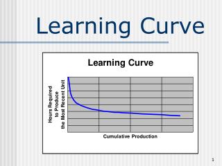
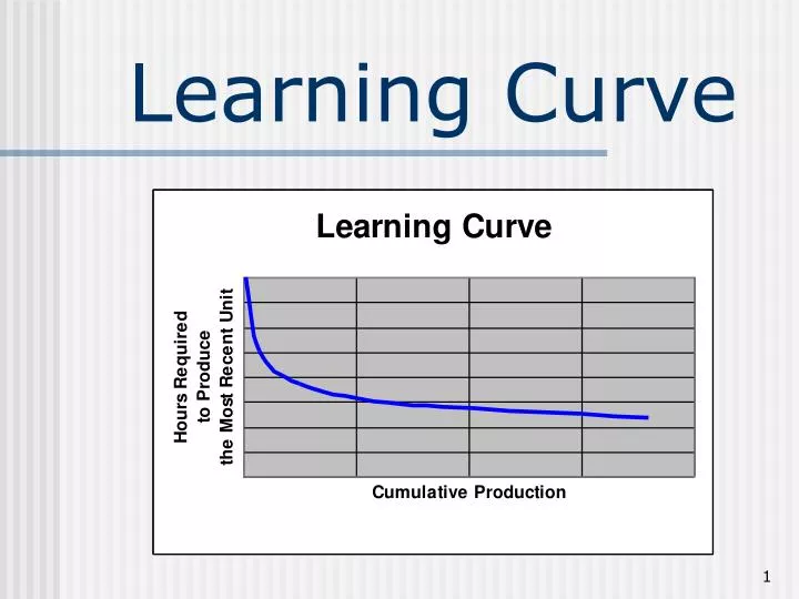
Example • Consider a product with the following data about the hours of labor required to produce a unit: • Hours required to produce 1-st unit: 100 • Hours required to produce 10-th unit: 48 • Hours required to produce 25-th unit: 35 • Hours required to produce 75-th unit: 25 • Hours required to produce 200-th unit: 18 As more and more units are produced, the hours of labor required to produce the most recent unit is lower and lower.
Reasons for Continual Decease in the Number of Hours Required to Produce the Most Recent Unit On the previous slide, we observed that, as more and more units are produced, the hours required to produce the most recent unit is lower and lower. What are some potential reasons why this occurs?
What happens whencumulative production doubles? The concept of a Learning Curve is motivated by the observation (in many diverse production environments) that, each time the cumulative production doubles, the hours required to produce the most recent unit decreases by approximately the same percentage. • For example, for an 80% learning curve, • If cumulative production doubles from 50 to 100, then the hours required to produce the 100-th unit is 80% of that for the 50-th unit. • If cumulative production doubles from 100 to 200, then the hours required to produce the 200-th unit is 80% of that for the 100-th unit.
The Functional Formof a Learning Curve • To model the behavior described in the previous slides, we proceed as follows: • Let x = cumulative production • y = hours required to produce the x-th unit • Then,y = ax-b • where a and b are parameters defined as follows: • a = hours required to produce the 1-st unit • b = a value related to the percentage associated with the Learning Curve
An 80% Learning Curve Assume that production of the first unit required 100 hours and that there is an 80% Learning Curve. Again, let x = cumulative production y = hours required to produce the x-th unit Then, mathematicians can show that the Learning Curve is y = 100x-0.322
A 70% Learning Curve Assume that production of the first unit required 100 hours and that there is an 70% Learning Curve. Again, let x = cumulative production y = hours required to produce the x-th unit Then, mathematicians can show that the Learning Curve is y= 100x-0.515
The Relationship Betweenb and p Recall that the functional form for a Learning Curve is y = ax-b The table below shows the relationship between the exponent b and p, the percentage associated with the Learning Curve:
The Relationship Betweenb and p (continued) There is a direct mathematical relationship between the exponent b in the equation y = ax-b and (p/100)%, where p is the percentage associated with the learning curve: For example, if p=75%, then For example, if b=0.737, then NOTE: e=2.7183… (never ending, like ¶) ln(x) is the exponent of e that yields x. That is, eln(x)=x
Operational Applicationof the Leaning Curve Assume that production of the 1-st unit required 100 hours, and assume that there is an 80% learning curve. Then, y = 100x-0.322. Also, assume that cumulative production to date is 150 units. The learning curve can be used to provide estimates of answers to questions about the production of the next 100 units.
Operational Application of a Leaning Curve (continued) Question 1: To produce the next 100 units, how many hours of labor will be required? Question 2: With a labor force of 6 workers each working 40 hours per week, how long will it take to produce then next 100 units? Question 3: To produce 100 units in 5 weeks with each worker working 40 hours per week, what should be the size of the labor force? Question 4: To produce 100 units in 5 weeks using a work force of 60 workers, how many hours per week should each worker work?
Effect of Sales’Annual Growth Rate • Assume that: • Three firms have the same 80% learning curve: y=100x-0.322 • During Year 1, all three firms sold 5000 units. • The three firms have respective annual growth rates in sales of 5%, 10%, and 20%. • Compare the three firms at the end of Year 4. Conclusion?
Strategic Applicationsof a Learning Curve Frequent Decreases in Selling Price. As the hours required to produce the most recent unit continually decreases, the cost to produce the unit continually decreases. Therefore, you can frequently decrease the selling price without decreasing total profit. Each decrease in selling price increases your market share, which in turn leads to a “faster ride” down the learning curve, which in turn makes it tougher for your competitors. Reinvest Increased Profits As the hours required to produce the most recent unit continually decreases, the cost to produce the unit continually decreases. Therefore, your profits increase. You can reinvest the incremental profit to improve the product or the production process, or you can reinvest the incremental profit in another area of the firm.
How do we determine the parameters of a Learning Curve? • From previous slides, we know that, to model a learning curve, we proceed as follows: • Let x = cumulative production • y = hours required to produce the x-th unit • Then, y = ax-b • where a and b are parameters defined as follows: • a = hours required to produce the 1-st unit • b = a value related to the percentage associated with the learning curve • For a given set of data, how do we determine the specific values of a and b?
Example For the Learning curve y=ax-b, how do we determine the specific values of a and b? We begin by taking the natural logs of both sides of y=ax-b. Note the linear relationship between ln(x) and ln(y). This suggests taking the natural logs of the data.
Example (continued) Note the approximate linear relationship between ln(Cumulative Production) and ln (Hours Required). We can use the statistical technique of Regression to determine the straight line that “best fits” the data.
Example (continued) Using Excel’s Regression Tool, we obtain ln(y) = 8.29642 – 0.23694 ln(x) Negative of Slope = 0.23694 Intercept=8.29642
Example (continued) From the previous slide, we know ln(y) = 8.29642 – 0.23694 ln(x) So, eln(y) = e[8.29642 – 0.23694 ln(x)] or, equivalently, the equation for the Learning Curve is y = 8.29642 x-0.23694
Example (continued) y = 8.29642 x-0.23694
Example (continued) y = 8.29642 x-0.23694 So, in our example, we have a Learning Curve that is close to but just below an 85% learning curve.
A “Not So Nice” Example In our example, there was a very close linear relationship between ln(Cumulative Production) and ln(Hours Required) This is NOT the typical situation. A more typical situation is shown on the next slide.
A “Not So Nice” Example(continued) Although the linear relationship in this example is not as strong as in the previous example, we proceed in the same manner.
A “Not So Nice” Example(continued) An approximate linear relationship such as the one below occurs for many products and services.