Using protein interaction networks to identify candidate disease genes in psychiatric illness.

1. Using protein interaction networks to identify candidate disease genes in psychiatric illness. Richard Adams, Psychiatric Genetics Lab, Medical Genetics Section, Molecular Medicine Centre, WGH, University of Edinburgh. richard.adams@ed.ac.uk Human genetics successful in identifying genetic causes of monogenic (Mendelian) disorders : - strong correlation between mutation and disease - mapping studies able to pinpoint susceptible region quite precisely - small number of candidate genes to study - reproducible results across populations. - >1000 disease genes identified to date Less successful in identifying genetic basis of complex (non-Mendelian) genetic disease - many mutations in many genes may contribute to the disease - often there is a high environmental influence - weak correlation between mutation and disease. - mapping studies often able to localise susceptible region only with 10s of Mb - hundreds of candidate genes - irreproducible results across populations - <10 undisputed disease genes identified to date

2. Bipolar disorder • - Bipolar disorder is a serious psychiatric disease (“manic depression”) • - Affects 1% of the population • - Family, twin and adoption studies indicate a genetic risk factor (50%). • - No molecular or cellular mechanism of the disease. • - “candidate gene” approach has not yielded breakthroughdue to the • irreproducibility of the results. • - little evidence of alterations in brain structure • - Experimental approach challenging: • - no disease model in experimental organisms. • - difficulty in obtaining tissue samples. • Many genomic regions implicated in BPAD predisposition • - many 00s of possible genes. • - currently impractical to study all simultaneously. • - how can we prioritize genes for further study? Schizophrenia • about 10 genes with multiple lines of evidence • most impact on the biology of the synapse: • receptors (CHRNA7, G72, GRM3) • synaptogenesis (DISC1, neuregulin, dysbindin, calcineurin) • Signal transduction ( RGS4)

3. F22 F59 F50 F48 1.2 2.2 2.0 8.5 Minimal Region I 12 11.3Mb 3.2 21 27 Minimal Region II Figure 2: Four families display linkage to chromosome 4p15-16. Minimal region I and II are defined by the regions where three of the four linkage signals overlap. Linkage studies identify a candidate region on chr 4p. • - approx. 9.5Mb is shared between 3 of the 4 families • 33 known genes in this region, only 1 obvious candidate, a dopamine receptor - no convincing • association shown to date .

4. Approaches to disease gene prediction Annotation based: e.g., GeneSeeker - assists in a candidate gene approach by searching multiple databases and finding genes based on user-provided query e.g., Bork group - associate pathological conditions with Gene Ontology terms. these assume some idea of the genes underlying the disease, or will find genes consistent with what is already known of the disease. e.g., POCUS - given 2 genomic regions, identifies genes sharing GO ids and protein domains makes no assumptions on protein function or expression. but results are dependent on extent of GO annotation. Sequence based: Ponting et al., - disease genes under represented in slowly evolving , intracellular widely expressed genes. Disease genes, in general have slightly different sequence characteristics (tend to be longer and more conserved). Use these differences for developing classifiers (e.g.,Prospectr).

5. Disease genes are significantly longer than “non-disease” genes (p < 4e-16). Disease genes All genes frequency Protein length(aa)

6. START Mouse homol >42% Has signal Peptide? Mouse homol >95% Gene length >997bp Gene length >563 Exons > 32 N Y N Y N Y N Y N Y N Y 0.827 -0.163 0.114 -0.315 -0.036 0.151 0.818 -0.026 0.029 -0.594 0.792 -0.014 Best paralog >78% Rata %id >59% 3’UTR < 647bp CDS len >704bp Hs/Mm Ka/Ks <0.195 N Y N Y N Y N Y N Y -0.57 0.008 0.344 -0.422 0.205 -0.044 -0.087 0.106 0.2 -0.034 GC > 37.5% N Y Mouse %id > 68.3% Worm %id >55% N Y N Y 0.213 -0.038 -0.492 0.015 0.027 -0.034 Prospectr, an alternating decision tree classifier

7. Improved approaches to predicting disease genes? Sequence based : + Hypothesis independent approach + Data available for all genes. + Possibility of discovering unexpected disease genes - do not take into account biological knowledge - predictions are not disease specific. • ideal approach would have information for all genes but would be hypothesis independent. • -Therefore large -scale protein interaction and expression data may be key.

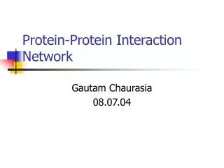
8. Protein interaction networks - key facts • Aggregation of multiple bimolecular interactions into • an undirected , “scale free” cyclic graph • Networks are not random : many sparsely connected proteins are linked through a smaller number of highly connected “hubs”. • Networks are also modular - <20 highly connected proteins loosely connected to rest of network. • Hubs are likely to be more ancient, conserved proteins. • Compared to random networks, any 2 nodes on average can be connected by shorter paths. • Can the properties of proteins in interaction networks be used to discriminate disease vs non-disease genes?

9. Clustering coefficient Neighbor count Articulation points Motif membership

10. Clustering coefficient ( 2n/k(k-1) ) Neighbor count Articulation points Motif membership

11. Clustering coefficient Neighbor count Articulation points Motif membership

12. Clustering coefficient Neighbor count (degree) Articulation points Motif membership

13. Clustering coefficient Neighbor count Articulation points Motif membership

14. Clustering coefficient Neighbor count Articulation points Motif membership

15. Sources of human protein interaction data…. Thought to be 40 000 - 200 000 pairwise interactions in humans… Experimental- literature (HPRD, BIND), 8802 proteins, 19000 interactions + “real” interactions + not all hi throughput - derived from many experimental approaches - nomenclature problems Predictions i) - extrapolated from lower organism high throughput data, 3890 proteins, 11 000 interactions (high quality), 11 000 proteins, 70 000 interactions (low quality) (Lehner and FraserGenome Biology 5 R63) +not entirely theoretical - only contains ancient proteins, no vertebrate specific proteins . ii) Extraploated from vertebrate interactions iii) -predicted from structural considerations (HPID) 20 000 proteins, 22 100 000 interactions. + probably contains most theoretically possible interactions. +good coverage of genome. - majority will be false positives, needs filters to be useful.

16. Dataset Features Lehner/ Fraser HPRD merge Nodes (proteins) 3890 8802 10 916 Edges (interactions) 11 000 19 000 26 000 Mean degree 5.2 4.7 5.9 Mean clust Coeff 0.11 0.14 0.12 Artic. Point count 780 (20%) 2100 (24%) 1632 (15%) Density 0.0015 0.0004 0.0005 Generating composite protein interaction sets • need to get as big a dataset as possible with as many interactions as possible • therefore have developed Perl modules to merge datasets from disparate sources • - modules are part of the BioPerl distribution • - deals with nomenclature issues when deciding if an interaction is common to • both datasets or not.

17. Comparing network properties of disease vs Non- disease genes. Database analysis L-F HPRD Merge D ND D ND D ND Articulation point % 20.2 19.8 23.8 24.6 18.2 15.3 median no. nbors 5.1 5.3 4.6 4.8 6.4 5.8 Median clust. Coeff.. 0.11 0.12 0.14 0.13 0.12 0.13 Small difference, little discrimination in classifier.

18. Identifying candidate disease genes by molecular triangulation (Krauthammer et al., PNAS 2004 101 15148-15153) • - Alzheimer’s Disease is a complex genetic disease with 4 known affective genes. • - use a custom protein interaction database derived from text-mining, with 3100 nodes and • 17000 interactions. • - assume that • 1 . AD related genes are clustered in a subnetwork of protein interactions, • 2 . Randomly selected seed genes are uniformly distributed around the network. • Use set of “seed” genes derived from expert list, or linkage results, or 4 known genes • - score each protein in network by how close it is to the seed genes. • proteins can be ranked by their scores • - proteins in expert lists can be objectively rated • - high scoring proteins can be picked out from others in a given linkage region

19. Method: Initalise: give seed genes an initial score: For each protein P in network: calculate distance to each seed gene. calculate score S for P where score  f(distance) increment P’s score by S next P To calculate significance: perform above algorithm 1000x using random seed gene selections: get score distribution for each node. P value for a given score S is the probability of exceeding that score in random selections e.g., if S  seed score/(distance +1): 5 2

20. Method: Initialise: give seed genes an initial score: For each protein P in network: calculate shortest path length to each seed gene (Djikstra). calculate score S for P where score  f(distance) increment P’s score by S next P To calculate significance: perform above algorithm 1000x using random seed gene selections: get score distribution for each node. P value for a given score S is the probability of exceeding that score in random selections 5/4 (1.25) 5 2

21. Method: Initalise: give seed genes an initial evidence-based score : For each protein P in network: calculate shortest path length to each seed gene (Djikstra). calculate score S for P where score  f(distance) increment P’s score by S next P To calculate significance: perform above algorithm 1000x using random seed gene selections: get score distribution for each node. P value for a given score S is the probability of exceeding that score in random selections 5/4 + 2/7 = 1.54 5 2

22. Method: Initalise: give seed genes an initial score: For each protein P in network: calculate shortest path length to each seed gene (Djikstra). calculate score S for P where score  f(distance) increment P’s score by S next P To calculate significance: perform above algorithm 1000x using random seed gene selections: get score distribution for each node. P value for a given score S is the probability of exceeding that score in random selections 2.33 1.54 2.00 2.25 5.5 3.17 2.9 3.25 2.67

23. Results of Krauthammer study • were able to rank expert list • - using 4 known genes as seeds, expert curated genes appeared higher rated than by chance • highlighted novel candidate genes for which some functional evidence exists. • produced a shortlist of 11 genes from 158 candidate genes from whole genome linkage study • . • Shortcomings: • - Only a limited set of protein interactions and proteins • Expert list used as a benchmark is not a “gold standard” and may be flawed. • No attempt to use different distance measures.

24. Identifying genes predisposing to BPAD / SCZ • unlike Alzheimer’s, we don’t have 4 definitively known genes . • currently testing how this approach works using the 10 strongest SCZ candidates • how well does this approach work for genes that may be more loosely connected • in a network? • - how well does assumption hold about clustering of seeds in a sub-network? • use a leave-one-out approach - how highly does the “left out” gene score? • can we enhance the concept of network distance? • e.g., giving edges a weight depending on the number of independent Shortest paths • between 2 nodes. • e.g., weighting edges where both proteins are known to exist in the brain (BIND). • e.g., calculating a Cartesian distance using a 3D network representation? • is there a way to model the expected score distribution of random seed genes? • as number of nodes increases, shortest path calculations become either very slow • or very memory intensive. • - this has to date been limiting for us, so far we have just prototyped code using a small network.