Download
1 / 21
210 likes | 327 Vues
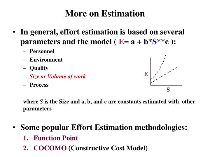
More on Estimation. In general, effort estimation is based on several parameters and the model ( E = a + b* S **c ): Personnel Environment Quality Size or Volume of work Process where S is the Size and a, b, and c are constants estimated with other parameters

E N D
More on Estimation • In general, effort estimation is based on several parameters and the model ( E= a + b*S**c ): • Personnel • Environment • Quality • Size or Volume of work • Process where S is the Size and a, b, and c are constants estimated with other parameters • Some popular Effort Estimation methodologies: • Function Point • COCOMO (Constructive Cost Model) E S
“simplified” Function Point • Proposed by Albrecht of IBM as an alternative metric to lines of code count for S, “size/comlexity” of product. • Based on 5 major areas and a complexity table of simple, average and complex set of weights as follows: simpleaveragecomplex • input 3 4 6 • output 4 5 7 • inquiry 3 4 6 • master files 7 10 15 • interfaces 5 7 10 • The Unadjusted Function Point is : • UFP = w*Inp + w2*Out + w3*Inq + w4*MastF +w5*Intf
Function Point (cont.) • 14 technical complexity factors are included, each valued between 0 and 5: • data communications • distributed data • performance criteria • heavy hardware usage • high transaction rates • online data entry • online updating • complex computations • ease of installation • ease of operation • portability • maintainability • end-user efficiency • reusability
Function Point (cont.) • The sum of 14 technical complexity factors can have values of 0 through 70. • The Total Complexity Factor(TCF) is defined as: • TCF = .65 + (.01 * Sum of 14 technical complexity factors) • TCF may have values of 0.65 through 1.35. • Finally, Function Point (FP) is defined as: • FP = UFP * TCF • For Cost and Productivity per FP, one may use “historical” data.
Simple Function Point Example • Consider the previous POWER function project and use Simple weights from the table : • 2 inputs, 1 output, 0 inquiry, 0 master file, and 0 interfaces • UFP = 3* 2 + 4*1 + 3*0 + 7*0 + 5*0 = 10 • consider the 14 complexity factors : 0-data comm; 0-distrib data; 0-perf criteria; 0-hardware usage; 0-transaction rate; 1-online data entry; 0-end user efficiency; 0-online update; 5-complex computation;0-reusability; 0-ease of install; 0-ease of operation; 0-portability; 1-maintainability: • TCF = .65 + (.01 * 7 ) = .72 • FP = UFP * TCF • FP = 10 * .72 • FP = 7.2 This is just the “size/complexity” (see next slide)
Function Point Example (cont.) • What does 7.2 function pointsmean in terms of schedule and cost estimates ? • One can receive guidance from IFPUG (International Function Point User Group) to get some of the $/FP or person-days/FP data. • With “old IBM services division” data of 20 function points per person month to perform “complete” development, 7.2 FP translates to approximately .36 person months or (22days * .36 = 7.9 person days) of work. • Assume $7k/person-month, .36 person months will cost about $2.5k.
Some Function Points Drawbacks • Requires “trained” people to perform estimates of work volume or product size, especially the 14 technical complexity factors. • While IFPUG may furnish some broader data, Cost and Productivity figures are different from organization to organization. • e.g. the IBM data takes into account of lots of corporate “overhead” cost • Some of the Complexity Factors are not that important or complex with today’s tools.
COCOMO Estimating Technique • Developed by Barry Boehm in early 1980’s who had a long history with TRW and government projects (initially, LOC based ) • Later modified into COCOMO II in the mid-1990’s (FP preferred but LOC is still used) • Assumed process activities : • Product Design • Detailed Design • Code and Unit Test • Integration and Test • Utilized by some but most of the software industry people still rely on experience and/or own company proprietary data. Note : Requirements not included!
COCOMO I Basic Form for Effort • Effort = A * B * (size ** C) • Effort = person months • A = scaling coefficient • B = coefficient based on 15 parameters • C = a scaling factor for process • Size = delivered source (K) lines of code
COCOMO I Basic form for Time • Time = D * (Effort ** E) • Time = total number of calendar months • D = A constant scaling factor for schedule • E = a coefficient to describe the potential parallelism in managing software development
COCOMO I • Originally based on 56 projects • Reflecting 3 modes of projects • Organic : less complex and flexible process • Semidetached : average project • Embedded : complex, real-time defense projects
3 Modes are Based on 8 Characteristics • Team’s understanding of the project objective 2. Team’s experience with similar or related project 3. Project’s needs to conform with established requirements 4. Project’s needs to conform with established interfaces 5. Project developed with “new” operational environments 6. Project’s need for new technology, architecture, etc. 7. Project’s need for schedule integrity 8. Project’s size range
COCOMO I • For the basic forms: • Effort = A * B *(size ** C) • Time = D * (Effort ** E) • Organic : A = 3.2 ; C = 1.05 ; D= 2.5; E = .38 • Semidetached : A = 3.0 ; C= 1.12 ; D= 2.5; E = .35 • Embedded : A = 2.8 ; C = 1.2 ; D= 2.5; E = .32
Coefficient B • Coefficient B is an effort adjustment factor based on 15 parameters which varied from very low, low, nominal,high, very highto extra high • B = “multiplicative product” of (15 parameters) • Product attributes: • Required Software Reliability : .75 ; .88; 1.00; 1.15; 1.40; • Database Size : ; .94; 1.00; 1.08; 1.16; • Product Complexity : .70 ; .85; 1.00; 1.15; 1.30; 1.65 • Computer Attributes • Execution Time Constraints : ; ; 1.00; 1.11; 1.30; 1.66 • Main Storage Constraints : ; ; 1.00; 1.06; 1.21; 1.56 • Virtual Machine Volatility : ; .87; 1.00; 1.15; 1.30; • Computer Turnaround time : ; .87; 1.00; 1.07; 1.15;
Coefficient B (cont.) • Personnel attributes • Analyst Capabilities : 1.46 ; 1.19; 1.00; .86; .71; • Application Experience : 1.29; 1.13; 1.00; .91; .82; • Programmer Capability : 1.42; 1.17; 1.00; .86; .70; • Virtual Machine Experience : 1.21; 1.10; 1.00; .90; ; • Programming lang. Exper. : 1.14; 1.07; 1.00; .95; ; • Project attributes • Use of Modern Practices : 1.24; 1.10; 1.00; .91; .82; • Use of Software Tools : 1.24; 1.10; 1.00; .91; .83; • Required Develop schedule : 1.23; 1.08; 1.00; 1.04; 1.10;
An example • Consider an average project of 10Kloc: • Effort = 3.0 * B * (10** 1.12) = 3 * 1 * 13.2 = 39.6 pm • Where B = 1.0 (all nominal) • Time = 2.5 *( 39.6 **.35) = 2.5 * 3.6 = 9 months • This requires an additional 8% more effort and 36% more schedule time for product plan and requirements: • Effort = 39.6 + (39.6 * .o8) = 39.6 + 3.16 = 42.76 pm • Time = 9 + (9 * .36) = 9 +3.24 = 12.34 months I am cheating here!
Try the POWER Function Example • POWER function was assumed to be 100 loc of C++ code, fairly simple (or Organic), and nominal for B factor: • Effort = 3.2 * 1 * ( .1 ** 1.05) = appr. 0.3 person- month • Time = 2.5 * ( .3 ** .38) = appr. 1.5 months • Note that while it takes only (.3 * 22 person days = 6.7 person days of effort), the total project duration will be 1.5 months.
Some COCOMO I concerns • Is our initial loc estimate accurate enough ? • Are we interpreting each parameter the same way ? • Do we have a consistent way to assess the range of values for each of the 15 parameters ?
COCOMO II • Effort performed at USC with many industrial corporations participating (still guided by Boehm) • Has a database of over 80 some projects • Early estimate, preferred to use Function Pointinstead of LOC for size; later estimate may use LOC for size. • Coefficient B based on 15 parameters for early estimate is “rolled” up to 7 parameters, and for late estimates use 17 parameters. • Now coefficient B is further expanded to 29 “factor”
Let’s look at Our 3 Estimates for “POWER” • Work Breakdown Structure and personal experience: • Effort : 5 person days • Time : 3 calendars (done in parallel) • Function Point and using IBM service division data: • Effort : 7.9 person days • Time : 7.9 calendar days (done with 1 person) • COCOMO I and using Organic, 100 loc, and nominal for all B factors: • Effort : 6.7 person days • Time : 1.5 calendar months
Other Estimation Models • There are many tools and models , but none seem to have dominated the software field. • Many practicing professionals still depend on personal and proprietary data. • Some other early models : • Walston-Felix • SLIM (commercial-proprietary)