Download
1 / 51
510 likes | 669 Vues
Science of the Dark Energy Survey. Josh Frieman Fermilab and the University of Chicago Astronomy 41100 Lecture 1, Oct. 1 2010. www.darkenergysurvey.org. The Dark Energy Survey. Blanco 4-meter at CTIO. Study Dark Energy using 4 complementary* techniques: I. Cluster Counts

E N D
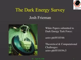
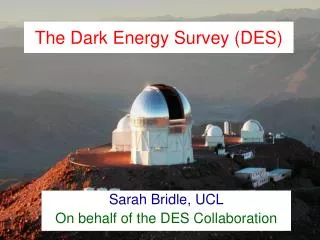
Science of the Dark Energy Survey Josh Frieman Fermilab and the University of Chicago Astronomy 41100 Lecture 1, Oct. 1 2010
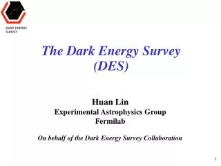
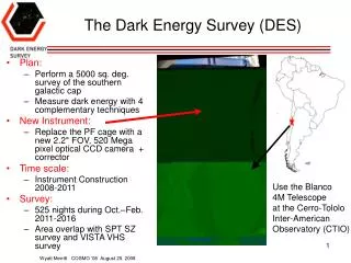
www.darkenergysurvey.org The Dark Energy Survey Blanco 4-meter at CTIO • Study Dark Energy using 4 complementary* techniques: I. Cluster Counts II. Weak Lensing III. Baryon Acoustic Oscillations IV. Supernovae • Two multiband surveys: 5000 deg2g, r, i, z, Y to 24th mag 15 deg2 repeat (SNe) • Build new 3 deg2 FOV camera and Data management sytem Survey 2012-2017 (525 nights) Camera available for community use the rest of the time (70%) *in systematics & in cosmological parameter degeneracies *geometric+structure growth: test Dark Energy vs. Gravity
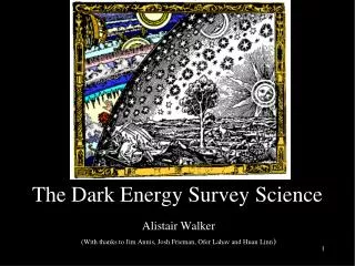
DES Instrument: DECam Mechanical Interface of DECam Project to the Blanco CCD Readout Filters Shutter Hexapod Optical Lenses Designed for improved image quality compared to current Blanco mosaic camera
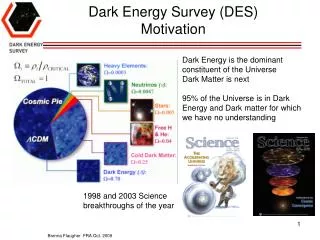
Cosmic Microwave Background Radiation The Universe is filled with a bath of thermal radiation COBE map of the CMB temperature On large scales, the CMB temperature is nearly isotropic around us (the same in all directions): snapshot of the young Universe, t ~ 400,000 years T = 2.728 degrees above absolute zero Temperature fluctuations T/T~105
The Cosmological Principle • We are not priviledged observers at a special place in the Universe. • At any instant of time, the Universe should appear ISOTROPIC (averaged over large scales) to all Fundamental Observers (those who define local standard of rest). • A Universe that appears isotropic to all FO’s is HOMOGENEOUS the same at every location (averaged over large scales).
The only modethatpreserves homogeneity and isotropy is overall expansion or contraction: Cosmic scale factor Model completely specified by a(t) and sign of spatial curvature
On average, galaxies are at rest in these expanding (comoving) coordinates, and they are not expanding--they are gravitationally bound. Wavelength of radiation scales with scale factor: Redshift of light: indicates relative size of Universe directly
Distance between galaxies: where fixed comoving distance Recession speed: Hubble’s Law (1929)
Modern Hubble Diagram Hubble Space Telescope Key Project Hubble parameter Freedman etal
Expansion Kinematics • Taylor expand about present epoch: where , and Recent expansion history completely determined by H0 and q0
How does the expansion of the Universe change over time? Gravity: everything in the Universe attracts everything else expect the expansion of the Universe should slow down over time
Cosmological Dynamics How does the scale factor of the Universe evolve? Consider a homogenous ball of matter: Kinetic Energy Gravitational Energy Conservation of Energy: Birkhoff’s theorem Substitute and to find K interpreted as spatial curvature in General Relativity M m d 1st order Friedmann equation
Cosmological Dynamics Spatial curvature: k=0,+1,-1 Friedmann Equations Density Pressure
Einstein-de Sitter Universe:a special case Non-relativistic matter: w=0, ρm~a-3 Spatially flat: k=0Ωm=1 Friedmann:
Empty Size of the Universe In these cases, decreases with time, : , expansion decelerates due to gravity Today -2/3 Cosmic Time
p = (w = 1) Accelerating Empty Size of the Universe Today Cosmic Time
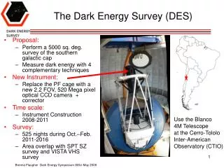
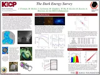
Log(distance) Discovery of Cosmic Acceleration from High-redshift Supernovae Type Ia supernovae that exploded when the Universe was 2/3 its present size are ~25% fainter than expected Accelerating = 0.7 = 0. m= 1. Not accelerating redshift
Cosmological Dynamics Friedmann Equations
Equation of State parameter w determines Cosmic Evolution Conservation of Energy-Momentum =Log[a0/a(t)]
Early 1990’s: Circumstantial Evidence The theory of primordial inflation successfully accounted for the large-scale smoothness of the Universe and the large-scale distribution of galaxies. Inflation predicted what the total density of the Universe should be: the critical amount needed for the geometry of the Universe to be flat: Ωtot=1. Measurements of the total amount of matter (mostly dark) in galaxies and clusters indicated not enough dark matter for a flat Universe (Ωm=0.2): there must be additional unseen stuff to make up the difference, if inflation is correct. Measurements of large-scale structure (APM survey) were consistent with scale-invariant primordial perturbations from inflation with Cold Dark Matter plus Λ.
Cosmic Acceleration This implies that increases with time: if we could watch the same galaxy over cosmic time, we would see its recession speed increase. Exercise 1: A. Show that above statement is true. B. For a galaxy at d=100 Mpc, if H0=70 km/sec/Mpc =constant, what is the increase in its recession speed over a 10-year period? How feasible is it to measure that change?
What is the evidence for cosmic acceleration? What could be causing cosmic acceleration? How do we plan to find out?
Cosmic Acceleration What can make the cosmic expansion speed up? The Universe is filled with weird stuff that gives rise to `gravitational repulsion’. We call this Dark Energy Einstein’s theory of General Relativity is wrong on cosmic distance scales. 3. We must drop the assumption of homogeneity/isotropy.
Cosmological Constant as Dark Energy Einstein: Zel’dovich and Lemaitre:
Recent Dark Energy Constraints Constraints from Supernovae, Cosmic Microwave Background Anisotropy (WMAP) and Large-scale Structure (Baryon Acoustic Oscillations, SDSS)
Components of the Universe Dark Matter: clumps, holds galaxies and clusters togetherDark Energy: smoothly distributed, causes expansion of Universe to speed up
assuming flat Univ. and constant w Only statistical errors shown
History of Cosmic Expansion • Depends on constituents of the Universe:
Cosmological Observables Friedmann- Robertson-Walker Metric: where Comovingdistance:
Exercise 2: A. For w=1(cosmological constant ) and k=0: Derive an analytic expression for H0t0 in terms of Plot B. Do the same, but for C. Suppose H0=70 km/sec/Mpc and t0=13.7 Gyr. Determine in the 2 cases above. D. Repeat part C but with H0=72.
Age of the Universe (H0/72) (flat)
Angular Diameter Distance • Observer at r =0, t0sees source of proper diameter D at coordinate distance r =r1 which emitted light at t =t1: • From FRW metric, proper distance across the source is so the angular diameter of the source is • In Euclidean geometry, so we define the D r =0 r =r1 Angular Diameter Distance:
Luminosity Distance • Source S at origin emits light at time t1 into solid angle d, received by observer O at coordinate distance r at time t0, with detector of area A: Proper area of detector given by the metric: Unit area detector at O subtends solid angle at S. Power emitted into d is Energy flux received by O per unit area is S A r
Include Expansion • Expansion reduces received flux due to 2 effects: 1. Photon energy redshifts: 2. Photons emitted at time intervals t1 arrive at time intervals t0: Luminosity Distance Convention: choose a0=1
Worked Example I For w=1(cosmological constant ): Luminosity distance:
Worked Example II For a flat Universe (k=0) and constant Dark Energy equation of state w: Luminosity distance: Note: H0dL is independent of H0
Dark Energy Equation of State Curves of constant dL at fixed z Flat Universe z =
Exercise 3 • Make the same plot for Worked Example I: plot curves of constant luminosity distance (for several choices of redshift between 0.1 and 1.0) in the plane of , choosing the distance for the model with as the fiducial. • In the same plane, plot the boundary of the region between present acceleration and deceleration. • Extra credit: in the same plane, plot the boundary of the region that expands forever vs. recollapses.
Bolometric Distance Modulus • Logarithmic measures of luminosity and flux: • Define distance modulus: • For a population of standard candles (fixed M), measurements of vs. z, the Hubble diagram, constrain cosmological parameters. flux measure redshift from spectra
Exercise 4 • Plot distance modulus vsredshift (z=0-1) for: • Flat model with • Flat model with • Open model with • Plot first linear in z, then log z. • Plot the residual of the first two models with respect to the third model
Log(distance) Discovery of Cosmic Acceleration from High-redshift Supernovae Type Ia supernovae that exploded when the Universe was 2/3 its present size are ~25% fainter than expected Accelerating = 0.7 = 0. m= 1. Not accelerating redshift
Distance and q0 Recall