Download
1 / 34
400 likes | 647 Vues
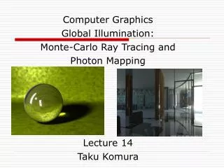
Computer Graphics -Global Illumination Techniques Lecture 14 Taku Komura. Before we go into the photon mapping. Let us summarize the techniques of rendering Local Illumination techniques Global Illumination techniques. Local Illumination methods .

E N D
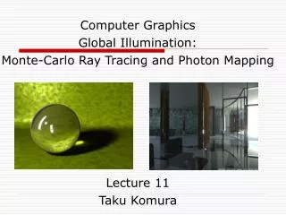
Computer Graphics -Global Illumination Techniques Lecture 14 Taku Komura
Before we go into the photon mapping... • Let us summarize the techniques of rendering • Local Illumination techniques • Global Illumination techniques
Local Illumination methods • Considers light sources and surface properties only. • Phong Illumination, Phong shading, Gouraud Shading • Using techniques like Shadow maps, shadow volume, shadow texture for producing shadows • Very fast • Used for real-time applications such as 3D computer games
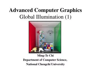
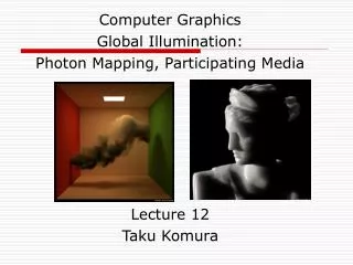
Lecture Notes #14 Global Illumination • Methods that simulate not only the direct illuminations but also the light indirect illuminations • Monte-Carlo ray tracing • Radiosity, Photon Mapping • Global illuminations can handle • Reflection (one object in another) • Refraction (Snell’s Law) • Shadows • Caustics under the same frame work • Requires more computation and is slow
Lecture Notes #14 Today : Global Illumination Methods • Radiosity (classic) • Photon Mapping (relatively new)
The Radiosity Method • View independent the rendering calculation does not have to be done although the viewpoint is changed • The basic method can only handle diffuse color → need to be combined with ray-tracing to handle specular light
The Radiosity Model • At each surface in a model the amount of energy that is given off (Radiosity) is comprised of • the energy that the surface emits internally, plus • the amount of energy that is reflected off the surface
The Radiosity Model(2) • The amount of incident light hitting the surface can be found by summing for all other surfaces the amount of energy that they contribute to this surface
Form Factor (Fij) • the fraction of energy that leaves surface i and lands on surface j • Between differential areas, it is • The overall form factor between i and j is
The Radiosity Matrix The radiosity equation now looks like this: The derived radiosity equations form a set of N linear equations in N unknowns. This leads nicely to a matrix solution:
Radiosity Steps: 1 - Generate Model 2 - Compute Form Factors 3 - Solve Radiosity Matrix 4 – Render • Only if the geometry of the model is changed must the system start over from step 1. • If the lighting or reflectance parameters of the scene are modified the system may start over from step 3. • If the view parameters are changed, the system must merely re-render the scene (step 4).
Radiosity Features: • The faces must be subdivided into small patches to reduce the artifacts • The computational cost for calculating the form factors is expensive • Quadratic to the number of patches • Solving for Bi is also very costly • Cannot handle specular light
Lecture Notes #14 Today : Global Illumination Methods • Radiosity (classic) • Photon Mapping (relatively new)
Photon Mapping • A fast, global illumination algorithm based on Monte-Carlo method • Casting photons from the light source, and saving the information of reflection when it hits a surface in the “photon map”, then render the results
Photon Mapping • A two pass global illumination algorithm • First Pass - Photon Tracing • Second Pass - Rendering
Photon Tracing • The process of emitting discrete photons from the light sources and tracing them through the scene • The goal is to populate the photon maps that are used in the rendering pass to calculate the reflected radiance at surfaces
Photon Emission • A photon’s life begins at the light source. • For each light source in the scene we create a set of photons and divide the overall power of the light source amongst them. • Brighter lights emit more photons
Review : Bidirectional Reflectance Distribution Function (BRDF) • The reflectance of an object can be represented by a function of the incident and reflected angles • This function is called the Bidirectional Reflectance Distribution Function (BRDF) • where E is the incoming irradiance and L is the reflected radiance
Photon Scattering • Emitted photons from light sources are scattered through a scene and are eventually absorbed or lost • When a photon hits a surface we can decide how much of its energy is absorbed, reflected and refracted based on the surface’s material properties
What to do when the photons hit surfaces • Attenuate the power and reflect the photon • For arbitrary BRDFs • Use Russian Roulette techniques • Decide whether the photon is reflected or not based on the probability • Reflect with full power
Arbitrary BRDF reflection • Can randomly calculate a direction and scale the power by the BRDF
Russian Roulette • If the surface is diffusive+specular, a Monte Carlo technique called Russian Roulette is used to probabilistically decide whether photons are reflected, refracted or absorbed. • Produce a random number between 0 and 1 • Determine whether to transmit, absorb or reflect in a specular or diffusive manner, according to the value
Diffuse and specular reflection • If the photon is to make a diffuse reflection, randomly determine the direction • If the photon is to make a specular reflection, reflect in the mirror direction
Photon Map • When a photon makes a diffuse bounce, the ray intersection is stored in memory • 3D coordinate on the surface • Color intensity • Incident direction • The data structure of all the photons is called Photon Map • The photon data is not recorded for specular reflections
Second Pass – Rendering • Finally, a traditional ray tracing procedure is performed by shooting rays from the camera • At the location the ray hits the scene, a sphere is created and enlarged until it includes N photons
Radiance Estimation • The radiance estimate can be written by the following equation
KD tree • The photon maps are classified and saved in a KD-tree • KD-tree : • dividing the samples at the median • The median sample becomes the parent node, and the larger data set form a right child tree, the smaller data set form a left child tree • Further subdivide the children trees • Can efficiently find the neighbours when rendering the scene
Precision • The precision of the final results depends on • the number of photons emitted • the number of photons counted for calculating the radiance
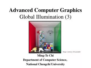
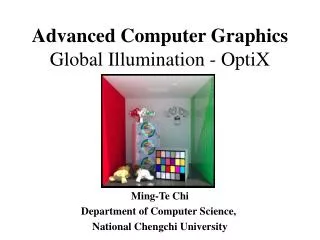
Simple Cornell box scene with 343 samplesper pixel and 10 million photons. Cornell box on acid with 343 samples perpixel and 10 million photons.
10,000 photons 1,000,000 photons 100,000 photons
Features of Photon Mapping • Can render caustics • Ray tracing cannot render caustics • Computationally efficient • Much more efficient than path-tracing
Why is photon mapping efficient? • It is a stochastic approach that estimates the radiance from a few number of samples • Kernel density estimation : operating directly on the samples, instead of creating a histogram of samples associated to the geometry
Summary • Local and Global Illuminations • Radiosity • Photon Mapping
Readings • Realistic Image Synthesis Using Photon Mapping by Henrik Wann Jensen • Global Illumination using Photon Maps (EGRW ‘96) Henrik Wann Jensen