Download
1 / 31
310 likes | 501 Vues
Parallel Algorithms. Sung Yong Shin TC Lab CS Dept. KAIST. Contents. 1. Background 2. Parallel Computers 3. PRAM 4. Parallel Algorithms. 1. Background. Von Neumann Machines sequential executing one instruction at a time

E N D
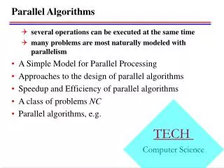
Parallel Algorithms Sung Yong Shin TC Lab CS Dept. KAIST
Contents 1. Background 2. Parallel Computers 3. PRAM 4. Parallel Algorithms
1.Background • Von Neumann Machines • sequential • executing one instruction at a time • Inherent limitation “ not faster than electrical signals ” 1 ft / 1 nanosecond ( 10-9 sec ) • Parallelism or Concurrency Carrying out many operations simultaneously • partition a complex problem in such a way that various parts of the work can be carried out independently and in parallel, and combine the results when all subcomputation are complete. • need parallel computers to support this approach.
Two approaches • Hardware-oriented • A parallel architecture of a specific kind is built. • The parallel algorithms for solving different problems are developed to make use of these hardware features to the best advantage. • Problem-oriented • Whether the parallel algorithms can truly enhance the speed of obtaining a solution to a given problem, or not. • If so, how much ?
Problems (i) The usefulness of parallel computers depends greatly on : • suitable parallel algorithms • parallel computer languages “ A major rethinking needed” (ii) Practical limitations by parallel computers “ too many factors to be considered” How to abstract ingredient from complex reality !!!
Which problems can be solved substantially faster using many processors rather than one processor ? • Nicholas Pippenger (1976) “ NC-class problems” ( Nick’s Class ) “ ultra-fast on a parallel computer with feasible amount of hardware” ( independent of the particular parallel model chosen ) • Inherent Parallelism probably not possible now but for the future !!! “ fascinating research topics” P P(n) processors NC (log n)m P-complete P = NC ?
Applications (needs ) • Computer vision / Image processing • Computer Graphics • Searching huge databases • Artificial Intelligence · · · · · · · ·
2. Parallel Computers SIMD ( Single Instruction Multiple Data Stream ) MIMD ( Multiple Instruction Multiple Data Stream ) What does SISD stand for ?
Program Result x+y Data Source x Function Unit y SISD
Program Result x+y x Add Function Unit y Data Source Result s+q s Add Function Unit q Result v+w Add v Function Unit w • SIMD • array processors • vector processors (pipelining)
Process3 Process4 Process1 Process2 Data Source Branch Function Unit NO Result x · y YES x Multiply Function Unit Data Source y Result w+v w Add Function Unit Data Source v Result s/q s Divide Function Unit Data Source q MIMD
Array Processors instructions (for multiple data) master slave slave slave Control Processor Arithmetic Processor Arithmetic Processor Arithmetic Processor PE Memory Memory Memory Memory Communication network
Identical Processors · · · P P P Interconnection network · · · M M M tightly coupled multiprocessors
P P P Identical Processing Elements ( PEs ) · · · M M M Interconnection network loosely coupled multiprocessors
Vector ( pipe-line ) processors functional unit Operand one Add exponents and multiply mantissas Compare components Align operands accordingly Determine normalization factor Result Operand two Normalize results Stage 1 Stage 2 Stage 3 Stage 4 Stage 5 A simplified pipeline for floating-point multiplication
3. PRAM (Parallel Random Access Machine) Processors (i) p general-purpose processors (ii) Each processor is connected to a large shared, random access memory M. (iii) Each processor has a private (or local) memory for its own computation. (iv) All communications among processors take place via the shared memory. (v) The input for an algorithm is assumed to be the 1stn memory cells, and output is to be placed in the 1st cell. (vi) All memory cells are initialized to be “0”. P1 P2 P3 Pp · · · Interconnection · · · M · · · 1 m Memory [A PRAM]
(vii) All processors run the same program. (viii) Each processor knows its own index. (ix) A PRAM program may instruct processors to do different things depending on their indices. write read computation three phases
Major Assumption (i) PRAM processors are synchronized !!! (1) processors begin each step at the same time. (2) All the processors that write at any step write at the same time. (ii) Any number of processors may read the same memory cell concurrently !!!
Variants of PRAM’s CREW ( Concurrent Read Exclusive Write ) CRCW ( Concurrent Read Concurrent Write ) – Common-write – Priority-write Why not EREW ? yes, if you want !!!
Other Models [Other parallel architectures] (a) A hypercube (dimension = 3) (b) A bounded degree network (degree = 4) ··· ··· · · · · · · · · · · · · · · · · (c) Octree model
4. Parallel Algorithms • Binary Fan-in Technique • Matrix multiplication • Handling write conflicts • Merging & Sorting
Binary Fan-in Technique P7 P5 P3 P1 x1 Read Read Compute Write Read Compute Write Read Compute Write x7 x3 x5 read x8 x2 x4 x6 comparison write save M[1] = max [A parallel tournament] ( finding Max )
Processors: Step 0 read M[i] into big Step 1 read M[i+1] into temp big := max (big, temp) write big Step 2 read M[i+2] into temp big := max (big, temp) write big Step 3 read M[i+4] into temp big := max (big, temp) write big P1 P2 P3 P4 P5 P6 P7 P8 M 16 12 1 17 23 19 4 8 16 12 1 17 23 19 4 8 M 16 12 1 17 23 19 4 8 12 1 17 23 19 4 8 – 16 12 17 23 23 19 8 8 M 16 12 17 23 23 19 8 8 17 23 23 19 8 8 – – 17 23 23 23 23 19 8 8 M 17 23 23 23 23 19 8 8 23 19 8 8 – – – – 23 23 23 23 23 19 8 8 M 23 23 23 23 23 19 8 8 max [A tournament example showing the activity of all the processors.]
read M[i] into big ; incr := 1 ; write – { some very small value } into M[n+i] ; for step := 1 to lg n do read M[i+incr] into temp ; big := max (big, temp) ; incr := 2 * incr ; write big into M[i] end { for } O( log n ) using n/2 processors no write conflicts
Matrix Multiplication O(n) using n2 processors What if using n3 processors ? O( log n ) Why ?
Handling write conflict Algorithm:Computing the or of n Bits Input : Bits x1, · · · · ,xn in M[1],· · · ·, M[n]. Output : x1 · · · · xn in M[1]. Pireads xi from M[i] ; If xi=1, then Pi writes 1 in M[1]. O(1) using n processors write conflict !!! CRCW – Common-write – Priority-write
Fast algorithm for finding Max Initial memory contents (n = 4). Input loser 2 7 3 6 0 0 0 0 8 1 P14 After Step 2 P13 P12 P23 P24 P34 1 1 1 1 1 1 2 7 3 6 1 0 1 1 P23 After Step 3 7 7 [Example for the fast max-finding algorithm] O(1) using processors common-write
Algorithm : Finding the Largest of n Keys Input : n keys x1, x2,···, xn, initially in memory cells M[1], M[2],···, M[n] (n>2). Output : The largest key will be left in M[1]. Comment : For clarity, the processors will be numbered Pi.j for 1 i j n. Step 1 Pi.j reads xi (from M[i]). Step 2 Pi.j reads xj (from M[j]). Pi.j compares xi and xj. Let k be the index of the smaller key. (If the keys are equal, let k be the smaller index.) Pi.j writes 1 in loser[k]. {At this point, every key other than the largest has lost a comparison. } Step 3 Pi.i+1 reads loser[i] ( and P1.n reads loser[n]) ; Any processor that read a 0 writes xi in M[1]. (P1.n would write xn.) { Pi.i+1 already has xi in its local memory ; P1.n has xn. }
Merging and Sorting merging P1 Pn Pn/2+1 Pn/2 x1 xn/2 yn y1 · · · · · · M[1] M[n] M[n/2] (a) Assignment of processors to keys. Pi yj xi >yj >xi <xi <yj (b) Binary search steps; Pi finds j such that yj-1<xi<yj. binary search Pi x1,…, xi-1 and y1,…, yj-1 (merged) xi M[i+j-1] (c) Output step. [Parallel merging] O(log n) using n processors no write conflict
Algorithm :Parallel Merging Input : Two sorted lists of n/2 keys each, in the first n cells of memory. Output : The merged list, in the first n cells of memory. Comment : Each processor Pihas a local variable x (if in/2) or y (if i>n/2) and other local variables for conducting its binary search. Each processor has a local variable position that will indicate where to write its key. Initialization : Pi reads M[i] into x (if in/2) or into y (if i>n/2). Pi does initialization for its binary search. Binary search steps : Processors Pi, for 1in/2, do binary search in M[n/2+1],…, M[n] to find the smallest j such that x<M[n/2+j], and assign i+j–1 to position. If there is no such j, Piassigns n/2+i to position. Processors Pn/2+i, for 1in/2, do binary search in M[1],…, M[n/2] to find the smallest j such that y<M[j], and assign i+j–1 to position. If there is no such j, Pi assigns n/2+i to position. Output step : Each Pi(for 1in) writes its key (x or y) in M[position].
Break the list into two halves. Sort the two halves (recursively). Merge the two sorted halves. Algorithm : Sorting by Merging Input : A list of n keys in M[1],…,M[n]. Output : The n key sorted in nondecreasing order in M[1],…,M[n]. Comment : The indexing in the algorithm is easier if the number of keys is a power of 2, so the first step will “pad” the input with large keys at the end. We still use only n processors. Piwrites (some large key) in M[n+i] ; for t := 1 to lg n do k := 2t-1 ; { the size of the lists being merged } Pi,…, Pi+2k-1 merge the two sorted lists of size k beginning at M[i]; end { for } O((log n)2) using n processors