Download
1 / 18
180 likes | 328 Vues
A Global Observing System for Monitoring and Prediction of Sea L evel C hange Lee -Lueng Fu COSPAR, 2014, Moscow Jet Propulsion Laboratory California Institute of Technology. Evolution of Earth Observation from Space. 1970-1990: Exploration

E N D
A Global Observing System for Monitoring and Prediction of Sea Level Change Lee-Lueng Fu COSPAR, 2014, Moscow Jet Propulsion Laboratory California Institute of Technology
Evolution of Earth Observation from Space • 1970-1990: Exploration • Weather satellites (TIROS, Nimbus, NOAA series, Meteor, Meteosat,…) • Land imaging (Landsat, SPOT, …) • Ocean observations (Seasat, Geosat,..) • Advanced measurement (UARS, T/P, ERS, …) • 1990-2010: Earth System Science • EOS (Terra, Aqua, Aura) • Envisat, TRMM • A-Train (Cloudsat, Calipso, GCOM-W, etc)
The Bretherton Diagram set the stage of Earth System Science
The A-Train example of an observing system The satellites are in a polar orbit, crossing the equator northbound at about 1:30 p.m. local time, within seconds to minutes of each other.
Earth System Science Approach to the Sea Level Problem lidar scatterometry altimetry InSAR River discharge Reference frame gravimetry In-situ Adapted from Church et al (2013)
Challenges • Understand the processes • Regional variability • Assessment and projection • Calibration and continuity IPCC AR5
Altimetric record of the global mean sea level Nerem et al, 2013
Global sea level change in terms of ocean heat and ice melt altimetry GRACE Argo Altimetry –GRACE Llovel et al., 2014
Detection of the rate change of global mean sea level • Altimetry: 2.8 +/- 0.4 mm/yr • The dominant error is tide gauge calibration owing to land motions. The time scale is much longer than decadal. • GRACE: 2.0 +/- 0.4 mm/yr • The dominant error is due to GIA correction with time scale much longer than decadal. • When calculating the rate change on decadal time scale, the long time scale errors are canceled, leading to 0.07 mm/yr for altimetry and 0.1 mm/yr for GRACE. • This allows detection of rate change of sea level of 0.28 mm/yr/decade and the rate change of the mass component of 0.4 mm/yr/decade, at 95% confidence.
Steric sea level and ocean warming • The standard error for the full-depth steric sea level rate is sqrt(0.072 + 0.12), or 0.12 mm/yr, comparable to the error estimated from Argo for the upper 2000 m(0.15 mm/yr) • This allows detection of rate change of steric sea level of 0.24 mm/yr/decade at 68% confidence, or 0.48 mm/yr/decade, ~50% of the signal, at 95 % confidence. • The rate of steric sea level can be related to the rate of ocean heat storage: • α = coefficient of thermal expansion • cp=specific heat at constant pressure; • q’=heat content anomaly/unit volume • If the warming is concentrated at the surface layer, then • Q’= ocean warming rate at W/m2
Regional variability: small long-term trends imbedded in large cyclic natural variability Willis et al (2011)
Decadal Sea Level Change in the Pacific Ocean Hamlington et al., 2013
The Effects of the Pacific Decadal Oscillation Hamlington et al., 2013
The length of time (in years) required for determining the trend of sea level change with an accuracy of 1 mm/yr. from 5 (deep blue) to 100 years (deep red). Hughes and Williams, 2011
A projection of sea level change from 2000 to 2100 Slangen et al (2011)
10 11 12 13 14 15 16 17 18 19 20 22 HY-2B China CRYOSAT-2 Europe SARAL/AltiKaFrance/India Jason-CS Europe/USA Sentinel-3B Europe SWOT USA/France Jason-2Europe/USA GLOBAL ALTIMETER MISSIONS Launch Date 08 09 21 Reference Missions - Higher Accuracy/Medium Inclination Jason-3 Europe/USA Complementary Missions - Medium Accuracy/Higher Inclination Sentinel-3A Europe Sentinel-3C/D HY-2A Operating Approved Proposed sw 24may11
Cross calibration between TOPEX/Poseidon and Jason-1 SSH Difference Before cm After cm Bonnefond and Haines, 2008
Conclusions • Among the suite of space-borne Earth observations, a system of measurements emerge to form an observing system for monitoring global sea level change. • The system allows the separation of the effect of ocean heat from that of melting ice, providing key information for estimating future sea level change and ocean warming. • The system provides cross-cutting information in oceanography, glaciology, meteorology, and geodesy to close the budget of sea level change. • International science teams have been established to assimilate the observations for making projection of future sea level change. Geodesy altimetry InSAR Argo Scientists & engineers Modeling