Download
1 / 77
860 likes | 1.31k Vues
Chapter 7 Localization & Positioning. Means for a node to determine its physical position with respect to some coordinate system (50, 27) or symbolic location (in a living room) Using the help of Anchor nodes that know their positions Directly adjacent nodes Over multiple hops.

E N D
Chapter 7Localization & Positioning Jang Ping Sheu
Means for a node to determine its physical position with respect to some coordinate system (50, 27) or symbolic location (in a living room) Using the help of Anchor nodes that know their positions Directly adjacent nodes Over multiple hops Goals of this chapter Jang Ping Sheu
7.1 Properties of localization and positioning procedures 7.2 Possible approaches 7.3 Mathematical basics for the lateration problem 7.4 Positioning in multi-hop environments 7.5 Positioning assisted by anchors Outline Jang Ping Sheu
Physical position versus logical location Coordinate system: position Symbolic reference: location Absolute versus relative coordinate Centralized or distributed computation Localized versus centralized computation Accuracy and precision: Accuracy: how close is an estimated position to the real position? Precision: the ratio with which a given accuracy is reached Scale (indoors, outdoors, global, …) Limitations: GPS for example, does not work indoors Costs: time, space, and energy consumption 7.1 Properties of localization and positioning procedures Jang Ping Sheu
Proximity A node wants to determine its position or location in the proximity of an anchor (Tri-/Multi-) lateration and angulation Lateration :when distances between nodes are used Angulation: when angles between nodes are used Scene analysis The most evident form of it is to analyze pictures taken by a camera Other measurable characteristic ‘fingerprints’ of a given location can be used for scene analysis e.g., RADAR Bounding box to bound the possible positions of a node 7.2 Possible approaches Jang Ping Sheu
Using information of a node’s neighborhood Exploit finite range of wireless communication e.g., easy to determine location in a room with infrared (room number announcements) Proximity (range-free approach) Jang Ping Sheu
(Tri-/Multi-)lateration and angulation Using geometric properties Lateration: distances between entities are used Angulation: angle between nodes are used Trilateration and triangulation (range-based approach) Jang Ping Sheu
To use (multi-)lateration, estimates of distances to anchor nodes are required. This ranging process ideally leverages the facilities already present on a wireless node, in particular, the radio communication device. The most important characteristics are Received Signal Strength Indicator (RSSI), Time of Arrival (ToA), and Time Difference of Arrival (TDoA). Trilateration and triangulation (cont.)Determining distances Jang Ping Sheu
Send out signal of known strength, use received signal strength and path loss coefficient to estimate distance Distance estimation RSSI (Received Signal Strength Indicator) Jang Ping Sheu
Problem: Highly error-prone process : Caused by fast fading, mobility of the environment Solution: repeated measurement and filtering out incorrect values by statistical techniques Cheap radio transceivers are often not calibrated Same signal strength result in different RSSI Actual transmission power different from the intended power Combination with multipath fading Signal attenuation along an indirect path is higher than along a direct path Solution: No! Distance estimationRSSI (cont.) Jang Ping Sheu
Distance estimationRSSI (cont.) PDF PDF Distance Signal strength Distance PDF of distances in a given RSSI value Jang Ping Sheu
Use time of transmission, propagation speed Problem: Exact time synchronization Usually, sound wave is used But propagation speed of sound depends on temperature or humidity Distance estimation ToA (Time of arrival ) Jang Ping Sheu
Use two different signals with different propagation speeds Compute difference between arrival times to compute distance Example: ultrasound and radio signal (Cricket System) Propagation time of radio negligible compared to ultrasound Problem: expensive/energy-intensive hardware Distance estimationTDoA (Time Difference of Arrival ) Jang Ping Sheu
RADAR system: Comparing the received signal characteristics from multiple anchors with premeasured and stored characteristics values. Radio environment has characteristic “fingerprints” The necessary off-line deployment for measuring the signal landscape cannot always be accommodated in practical systems. Scene analysis Jang Ping Sheu
Bounding Box The bounding box method proposed in uses squares instead of circles as in tri-lateration to bound the possible positions of a node. For each reference node i, a bounding box is defined as a square with its center at the position of this node (xi, yi), with sides of size 2di(where diis the estimated distance) and with coordinates (xi–di, yi–di) and (xi+di, yi+di). Jang Ping Sheu
Bounding Box(cont.) Using range to anchors to determine a bounding box Use center of box as position estimate B C d A Jang Ping Sheu
References N. Bulusu, J. Heidemann, and D. Estrin. “GPS-Less Low Cost Outdoor Localization For Very Small Devices,” IEEE Personal Communications Magazine, 7(5): 28–34, 2000. C. Savarese, J. Rabay, and K. Langendoen. “Robust Positioning Algorithms for Distributed Ad-Hoc Wireless Sensor Networks,” In Proceedings of the Annual USENIX Technical Conference, Monterey, CA, 2002. A. Savvides, C.-C. Han, and M. Srivastava. “Dynamic Fine-Grained Localization in Ad-Hoc Networks of Sensors,” Proceedings of the 7th Annual International Conference on Mobile Computing and Networking, pages 166–179. ACM press, Rome, Italy, July 2001. S. Simic and S. Sastry, “Distributed localization in wireless ad hoc networks,” UC Berkeley, Tech. rep. UCB/ERL M02/26, 2002. Jang Ping Sheu
7.3 Mathematical basics for the lateration problem Jang Ping Sheu
Solution with three anchors and correct distance values Assuming distances to three points with known location are exactly given Solve system of equations (Pythagoras!) (xi , yi) : coordinates of anchor pointi, ri : distance to anchor i (xu, yu) : unknown coordinates of node Jang Ping Sheu
Solution with three anchors and correct distance values (cont.) Jang Ping Sheu
Rewriting as a matrix equation: Trilateration as matrix equation Jang Ping Sheu
Solving with distance errors • What if only distance estimation available? • Use multiple anchors, overdetermined system of equations • Use (xu,yu) that minimize mean square error, • i.e, Jang Ping Sheu
Look at square of the of Euclidean norm expression (note that for all vectors v) Look at derivative with respect to x, set it equal to 0 Minimize mean square error Jang Ping Sheu
7.4 Positioning in multi-hop environments Jang Ping Sheu
Assume that the positions of n anchors are known and the positions of m nodes is to be determined, that connectivity between any two nodes is only possible if nodes are at most R distance units apart, and that the connectivity between any two nodes is also known The fact that two nodes are connected introduces a constraint to the feasibility problem – for two connected nodes, it is impossible to choose positions that would place them further than R away Connectivity in a multi-hop network Jang Ping Sheu
Multi-hop range estimation How to estimate range to a node to which no direct radio communication exists? No RSSI, TDoA, … But: Multi-hop communication is possible Jang Ping Sheu
Multi-hop range estimation (cont.) Idea 1: (DV-Hop) Start by counting hops between anchors then divide known distance Count Shortest hop numbers between all two nodes. Each anchors estimate hop length and propagates to the network. Node calculates its position based on average hop length and shortest path to each anchor. Jang Ping Sheu
DV Hop • L1 calculates average hope length : • So do L2 and L3 : • Node A uses trilateration to estimate it’s position by multiplying the average hope length of every received anchor to shortest path length it assumed. Jang Ping Sheu
DV-Distance • Idea 2: If range estimates between neighbors exist, use them to improve total length of route estimation in previous method (DV-Distance) • Distance between neighboring nodes is measured using radio signal strength and is propagated in meters rather than in hops. • The algorithm uses the same method to estimate but shortest distance length are assumed. Jang Ping Sheu
Must work in a network which is dense enough DV-hop approach used the hop of the shortest path to approximately estimate the distance between a pair of nodes Drawback: Requires lots of communications Multi-hop range estimation (cont.) DV-Based Scheme anchor anchor Jang Ping Sheu
Number of anchors Euclidean method increase accuracy as the number of anchors goes up The “distance vector”-like methods are better suited for a low-ratio of anchors Uniformly distributed network Distance vector methods perform less well in non-uniformly networks Euclidean method is not very sensitive to this effect Discussion Jang Ping Sheu
7.5 Positioning assisted by anchors Jang Ping Sheu
By pure connectivity information Idea: decide whether a node is within or outside of a triangle formed by any three anchors However, moving a sender node to determine its position is hardly practical ! Solution: inquire all its neighbors about their distance to the given three corner anchors APIT (Approximate Point in Triangle) Jang Ping Sheu
APIT (cont.) Inside a triangle Irrespective of the direction of the movement, the node must be closed to at least one of the corners of the triangle A M C B Jang Ping Sheu
APIT (cont.) Outside a triangle: There is at least one direction for which the node’s distance to all corners increases A M B C Jang Ping Sheu
Approximation: Normal nodes test only directions towards neighbors APIT (cont.) Jang Ping Sheu
Grid-based Aggregation Narrow down the area where the normal node can potentially reside APIT (cont.) 2 1 anchor node normal node Jang Ping Sheu
MCL (Monte-Carlo Localization) Assumptions Time is divided into several time slots Moving distance in each time slot is randomly chosen from [0, Vmax ] Each anchor node periodically forwards its location to two-hop neighbors Notation R - communication range 2014/8/24 38 Jang Ping Sheu
MCL (cont.) Each normal node maintains 50 samples in each time slot Samples represent the possible locations The sample selection is based on previous samples Sample (x , y) must satisfy some constraints Located in the anchor constraints 2014/8/24 39 Jang Ping Sheu
MCL (cont.) Anchor constraints Near anchor constraint The communication region of one-hop anchor node ( near anchor ) Farther anchor constraint The region within ( R, 2R ] centered on two-hop anchor ( farther anchor ) Near anchor constraint Farther anchor constraint R R R A1 A1 N1 N1 N2 2014/8/24 40 Jang Ping Sheu
MCL (cont.)Environment Anchor node Normal node A4 A1 A2 A3 N1 2014/8/24 41 Jang Ping Sheu
MCL (cont.)Initial Phase Anchor node Normal node A4 N1 A1 A2 A3 Sample in the last time slot 2014/8/24 42 Jang Ping Sheu
MCL (cont.)Prediction Phase & Filtering Phase Anchor node Normal node Vmax A4 N1 R A1 R R A2 A3 Sample in this time slot Sample in the last time slot 2014/8/24 43 Jang Ping Sheu
MCL (cont.)Prediction Phase & Filtering Phase Anchor node Normal node Vmax A4 Vmax A1 R A2 Vmax A3 Sample in this time slot Sample in the last time slot N1 R R 2014/8/24 44 Jang Ping Sheu
MCL (cont.)Estimative Location Anchor node Normal node A4 N1 EN1 A1 A2 A3 Sample in this time slot Estimative position • the average of samples 2014/8/24 45 Jang Ping Sheu
MCL (cont.) Repeated Prediction Phase & Filter Phase Anchor node Normal node Vmax A4 A1 R A2 A3 Sample in this time slot Sample in the last time slot In the next time slot N1 2014/8/24 46 Jang Ping Sheu
There are three phases in the DRLS algorithm. Phase 1 – Beacon exchange Phase 2 – Using improved grid-scan algorithm to get initial estimative location Phase 3 – Refinement DRLS Distributed Range-Free Localization Scheme Jang Ping Sheu
Beacon exchange via two-hop flooding DRLS (cont.)Beacon Exchange Normal node A4 Near anchor Farther anchor N3 A3 A1 N2 A2 N1 Jang Ping Sheu
DRLS (cont.)Improved Grid-Scan Algorithm up side right side left side down side • Calculate the overlappingrectangle N A3 A1 Anchor node A2 Normal node Jang Ping Sheu
DRLS (cont.)Improved Grid-Scan Algorithm Divide the ER into small grids The initial value of the grid is 0 0 0 0 0 A3 0 0 N 0 0 0 0 A1 0 0 A2 0 0 0 0 Anchor node Normal node Estimative location Jang Ping Sheu