Download
1 / 16
200 likes | 476 Vues
Facility Location Decisions. Classifying location decisions Driving force (critical factor - traffic, labor rates, emergency facilities, obnoxious facilities) Number of facilities Discrete vs. continuous choices Data aggregation Time Horizon. Facility Location.

E N D
Facility Location Decisions • Classifying location decisions • Driving force (critical factor - traffic, labor rates, emergency facilities, obnoxious facilities) • Number of facilities • Discrete vs. continuous choices • Data aggregation • Time Horizon
Facility Location • Rent Curve - The rent of land is a decreasing function of the distance to the market • Weight gaining vs. weight losing industries • Weight losing should locate close to raw materials • Weight gaining should locate close to market • Tapered (concave) transportation costs • The derivative of total transportation cost is non-increasing with the distance to the market (holds for inbound and outbound costs) • Optimal solution will always locate either at raw materials or at market (extreme point solution)
Single Facility Location Model • This model assumes a known set, I, of source and demand points, each with known demand volumes, Vi, and transportation rates, Ri. • The objective is to locate the facility at the point that minimizes total transportation cost, TC: • Let di denote the distance from the facility to demand point i. • Min • subject to: • The decision variables are the coordinates of the facility • Xi, Yi denote the coordinates of demand point i.
Single Facility Location Model • Differentiating TC w.r.t. and setting the result equal to zero gives the ‘center of gravity’:
Single Facility Location Model • Note however, that are given in terms of di, which is a function of • An algorithm that will converge to the optimal • This continuous problem is often called the Weber problem • These problems are restrictive because they assume continuity of location and straight-line distances • Also, only variable distance related costs are considered
General Facility Location Model • The general facility location problem considers the simultaneous location of a number of facilities • Notation: • I - Set of customers, indexed by i. • J - Set of facilities, indexed by j. • di - demand of customer i. • cij - cost of transporting a unit from facility j to customer i. • Fj - fixed cost of creating facility j. • xij - variable for flow from facility j to customer i. • Yj - binary variable that equals 1 if we create facility j, 0 otherwise • sj - capacity of facility j.
Location Decisions and Risk Pooling • Suppose we must serve n independent markets with a single product, and each market has average demand per period of D and standard deviation (we neglect lead times for simplicity) • Assume we have a service level policy to ensure that the probability of not stocking out in each period equals • Suppose we serve each market using a single inventory stocking location. • The standard deviation of demand as seen by the single stocking location in each period equals • If demand is normally distributed, the safety stock required at the single location equals z
Location Decisions and Risk Pooling • Suppose, at the other extreme, we place an inventory stocking location in each of the n markets • Each stocking location will need to hold z to meet the service level requirement • The system-wide safety stock equals zn> z • This example illustrates the risk-pooling effects of location decisions • The more stocking locations we have, the more duplication in safety stock we have • The single location, however, will incur the maximum transportation costs, while n locations should minimize the transportation costs
Location Decisions and Risk Pooling • The safety stock costs and transportation costs are at odds with each other • We need to strike a balance between the two • Models for this decision are currently limited (Prof. Shen has worked on a model that addresses this tradeoff) • However, this simple analysis can provide strong insights • If inventory costs dominate transportation costs (as in expensive computing chips), we are driven to have less stocking points; if transport costs dominate (as in coal), then we are driven to have more stocking locations • One thing not included in the analysis is delivery lead time and its impact on service levels – obviously more locations closer to markets can respond much more quickly to customers
Supply Chain Design Model • The objective of this model is to determine the warehouse and plant configuration that minimizes total costs for production and distribution of multiple products. • Based on Geoffrion and Graves, 1974, “Multicommodity distribution system design by Benders decomposition,” Management Science, v20, n5. (see Tech. Suppl., Ch. 13) • Notation: • i - index for commodities • j - index for plants • k - index for warehouses • l - index for customer zones
Supply Chain Design Model • Notation (continued): • Sij - production capacity for commodity i at plant j. • Dil - demand for commodity i in customer zone l. • - min and max total throughput for warehouse k. • fk - fixed part of annual costs for owning and operating warehouse k. • vk - variable unit cost of throughput for warehouse k. • Cijkl - average unit cost of producing, handling, and shipping commodity i from plant j through warehouse k to customer zone l. • Xijkl - amount of commodity i flowing from plant j through warehouse k to customer zone l. • ykl - binary variable = 1 if warehouse k serves customer zone l, 0 otherwise • zk - binary variable = 1 if warehouse k is open, 0 otherwise.
Network Planning • Network planning refers to assessing or reassessing the configuration of facilities, commodities, and flows currently used to satisfy demand • Network planning data checklist: • List of all products • Customer, stocking point, and source point locations • Demand by customer location • Transportation rates • Transit times, order transmittal times, and order fill rates • Warehouse rates and costs • Purchasing/production costs • Shipment sizes by product • Inventory levels by location, by product, control methods • Order patterns by frequency, size, season, content • Order processing costs and where they are incurred
Network Planning • Data Checklist (continued): • Capital cost • Customer service goals • Available equipment and facilities and their capacities • Current distribution patterns (flows) • Note that many of these are decision variables • Accumulating these data usually results in improvements by uncovering anomalies • We must decide our network design strategy: • Specify minimum service levels • Specify shortage costs and minimize cost • Levels of acceptable aggregation of demand • Optimization vs. heuristic methods • Which areas require the most accuracy and attention?