Download
1 / 28
280 likes | 412 Vues
Modern Physics 6a – Intro to Quantum Mechanics Physical Systems, Thursday 15 Feb. 2007, EJZ. Plan for our last four weeks: week 6 (today), Ch.6.1-3: Schr ö dinger Eqn in 1D, square wells week 7, Ch.6.4-6: Expectation values, operators, quantum harmonic oscillator, applications

E N D
Modern Physics 6a – Intro to Quantum MechanicsPhysical Systems, Thursday 15 Feb. 2007, EJZ • Plan for our last four weeks: • week 6 (today), Ch.6.1-3: Schrödinger Eqn in 1D, square wells • week 7, Ch.6.4-6: Expectation values, operators, quantum harmonic oscillator, applications • week 8, Ch.7.1-3: Schrödinger Eqn in 3D, Hydrogen atom • week 9, Ch.7.4-8: Spin and angular momentum, applications
Outline – Intro to QM • How to predict a system’s behavior? • Schrödinger equation, energy & momentum operators • Wavefunctions, probability, measurements • Uncertainty principle, particle-wave duality • Applications
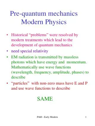
How can we describe a system and predict its evolution? Classical mechanics: Force completely describes a system: Use F=ma = m dp/dt to find x(t) and v(t). Quantum mechanics: Wavefunction y completely describes a QM system
Energy and momentum operators From deBroglie wavelength, construct a differential operator for momentum: Similarly, from uncertainty principle, construct energy operator:
Energy conservation Schroedinger eqn. E = T + V Ey = Ty + Vy where y is the wavefunction and operators depend on x, t, and momentum: Solve the Schroedinger eqn. to find the wavefunction, and you know *everything* possible about your QM system.
Schrödinger Eqn We saw that quantum mechanical systems can be described by wave functions Ψ. A general wave equation takes the form: Ψ(x,t) = A[cos(kx-ωt) + i sin(kx-ωt)] = e i(kx-ωt) Substitute this into the Schrodinger equation to see if it satisfies energy conservation.
Wave function and probability Probability that a measurement of the system will yield a result between x1 and x2 is
Measurement collapses the wave function • This does not mean that the system was at X before the measurement - it is not meaningful to say it was localized at all before the measurement. • Immediately after the measurement, the system is still at X. • Time-dependent Schrödinger eqn describes evolution of y after a measurement.
Exercises in probability: quantitative 1. Probability that an individual selected at random has age=15? 2. Most probable age? 3. Median? 4. Average = expectation value of repeated measurements of many identically prepared system: 5. Average of squares of ages = 6. Standard deviation s will give us uncertainty principle...
Exercises in probability: uncertainty Standard deviation s can be found from the deviation from the average: But the average deviation vanishes: So calculate the average of the square of the deviation: Exercise: show that it is valid to calculate s more easily by: HW: Find these quantities for the exercise above.
Expectation values Most likely outcome of a measurement of position, for a system (or particle) in state y: Most likely outcome of a measurement of position, for a system (or particle) in state y:
Uncertainty principle Position is well-defined for a pulse with ill-defined wavelength. Spread in position measurements = sx Momentum is well-defined for a wave with precise l. By its nature, a wave is not localized in space. Spread in momentum measurements = sp We saw last week that
Particles and Waves Light interferes and diffracts - but so do electrons! e.g. in Ni crystal Electrons scatter like little billiard balls - but so does light! in the photoelectric effect
Applications of Quantum mechanics Blackbody radiation: resolve ultraviolet catastrophe, measure star temperatures Photoelectric effect: particle detectors and signal amplifiers Bohr atom: predict and understand H-like spectra and energies Structure and behavior of solids, including semiconductors Scanning tunneling microscope Zeeman effect: measure magnetic fields of stars from light Electron spin: Pauli exclusion principle Lasers, NMR, nuclear and particle physics, and much more... Sign up for your Minilectures in Ch.7
Part 2: Stationary states and wells • Stationary states • Infinite square well • Finite square well • Next week: quantum harmonic oscillator • Blackbody
Stationary states If evolving wavefunction Y(x,t) = y(x) f(t) can be separated, then the time-dependent term satisfies Everyone solve for f(t)= Separable solutions are stationary states...
Separable solutions: (1) are stationary states, because * probability density is independent of time [2.7] * therefore, expectation values do not change (2) have definite total energy, since the Hamiltonian is sharply localized: [2.13] (3) yi = eigenfunctions corresponding to each allowed energy eigenvalue Ei. General solution to SE is [2.14]
Show that stationary states are separable: Guess that SE has separable solutions Y(x,t) = y(x) f(t) sub into SE=Schrodinger Eqn Divide by y(x) f(t) : LHS(t) = RHS(x) = constant=E. Now solve each side: You already found solution to LHS: f(t)=_________ RHS solution depends on the form of the potential V(x).
Now solve for y(x) for various V(x) Strategy: * draw a diagram * write down boundary conditions (BC) * think about what form of y(x) will fit the potential * find the wavenumbers kn=2 p/l * find the allowed energies En * sub k into y(x) and normalize to find the amplitude A * Now you know everything about a QM system in this potential, and you can calculate for any expectation value
Infinite square well: V(0<x<L) = 0, V= outside What is probability of finding particle outside? Inside: SE becomes * Solve this simple diffeq, using E=p2/2m, * y(x) =A sin kx + B cos kx: apply BC to find A and B * Draw wavefunctions, find wavenumbers: kn L= np * find the allowed energies: * sub k into y(x) and normalize: * Finally, the wavefunction is
Square well: homework Repeat the process above, but center the infinite square well of width L about the point x=0. Preview: discuss similarities and differences Infinite square well application: Ex.6-2 Electron in a wire (p.256)
Everywhere: Ψ, Ψ’, Ψ’’continuous Outside: Ψ→ 0, Ψ’’ ~ Ψ because E<V0 (bound) Inside: Ψ’’ ~ - Ψ because V=0 (V-E < 0)
Which of these states are allowed? Outside: Ψ → 0, Ψ’’ ~ Ψ because E<V0 (bound) Inside: Ψ’’ ~ - Ψ because V=0 (V-E < 0)
Finite square well: • BC: Ψ is NOT zero at the edges, so wavefunction can spill out of potential • Wide deep well has many, but finite, states • Shallow, narrow well has at least one bound state
Summary: • Time-independent Schrodinger equation has stationary states y(x) • k, y(x), and E depend on V(x) (shape & BC) • wavefunctions oscillate as eiwt • wavefunctions can spill out of potential wells and tunnel through barriers