Download
1 / 40
410 likes | 500 Vues
MATH4248 Weeks 10-11. Topics: Motion of a particle on a surface, calculus, calculus of variations and Hamilton’s principle of stationary action, kinetic energy and Riemannian manifolds, inertial motion and geodesics, covariance, invariance, constants of motion, rigid body motion.

E N D
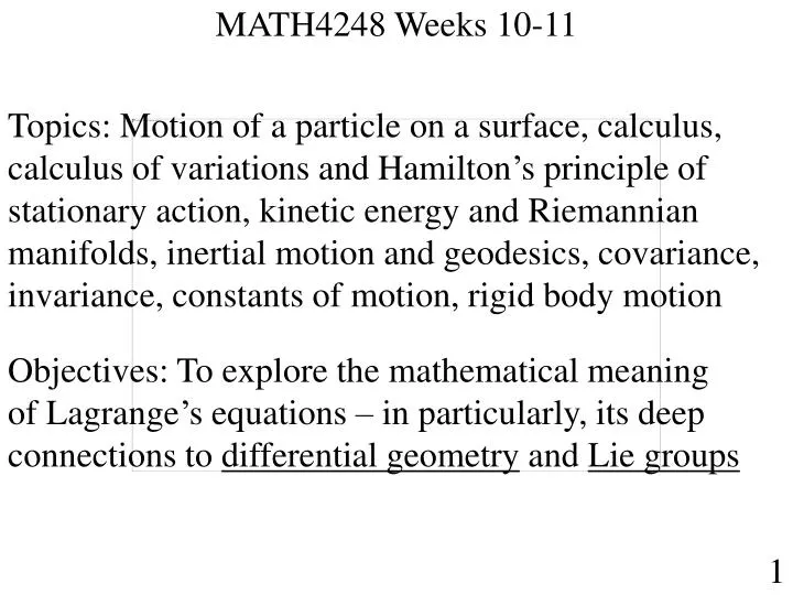
MATH4248 Weeks 10-11 Topics: Motion of a particle on a surface, calculus, calculus of variations and Hamilton’s principle of stationary action, kinetic energy and Riemannian manifolds, inertial motion and geodesics, covariance, invariance, constants of motion, rigid body motion Objectives: To explore the mathematical meaning of Lagrange’s equations – in particularly, its deep connections to differential geometry and Lie groups 1
MOTION OF A PARTICLE ON A SURFACE For a particle having mass m and constrained to move on the surface with generalized coordinates kinetic energy potential energy Lagrangian 2
MOTION OF A PARTICLE ON A SURFACE Euler-Lagrange equations generalized momenta and 3
CALCULUS Functions, their Graphs and Epigraphs Limits and Continuity Intermediate Values and Extreme Values Derivatives as Linear Approximations Integrals and The Fundamental Theorem of Calculus Derivative of Products and Integration by Parts Composition of Functions and the Chain Rule Extreme and Stationary Values Rolle’s Theorem and The Mean Value Theorem Convexity: Geometric and Algebraic Descriptions 6
FUNCTIONS, GRAPHS, AND EPIGRAPHS A function f : X Y is a ‘rule’ that assigns to every x in X (the domain) an element y in Y. The range of f, denoted by f(X), consists of all elements in Y having the form f(x), x in X The graph of a function f : X Y is the subset of the Cartesian Product that consists of all ordered pairs (x,f(x)), x in X. The epigraph of a function f : X R is the subset of the Cartesian Product that consists of all ordered pairs (x,y), x in X and Problem: Prove that 7
LIMITS Ref = Thomas’ Calculus Ref p.92 Let f(x) be defined on an open interval about , except possibly at itself. We way that f(x) approaches the limit L as x approaches and write if, for every number , there exists a such that for all x , Problem: Define limits for 8
CONTINUITY Ref. p.125 A function y=f(x) is continuous at an interior pointc of its domain if and is continuous at a left, right endpoint a, b of its domain if 9
THE INTERMEDIATE VALUE THEOREM Ref p.130 A function y=f(x) that is continuous on a closed interval [a,b] takes on every value between f(a) and f(b). In other words, if is any value between f(a) and f(b), then for some c in [a,b]. Problem: Interpret this in terms of the graph of f(x) 10
THE EXTREME VALUE THEOREM Ref p. 228 If f is continuous at every point of a closed interval I, then f assumes both an absolute maximum value M and an absolute minimum value m somewhere in I. That is, there are numbers and in I with The values m and M are called absolute or global extreme values. Problem: What is the range of f in terms of m and M ? 11
DERIVATIVES Ref p.147 For a function f : [a,b] R the derivative of the function f(x), with respect to the variable x, is the function whose value at x is provided that the limit exists. Equivalently, where the ratio o(h)/h 0 as h0. In a neighborhood of x in [a,b], f(x) is the constant approximation to f while the function is a linear approximation to f. 12
DERIVATIVES The derivative as a linear approximation provides the foundation for multivariable calculus With respect to the standard bases on the Euclidean spaces, h is a m x 1column vector and the derivative is an n x m matrix valued function on D. If n = 1 and the Euclidean dot or scalar product is considered then 13
INTEGRALS AND THE FUNDAMENTAL THEOREM OF CALCULUS Ref p. 354 Part 1. If f is continuous then Ref p. 358 Part 2. If f is continuous and then 14
DERIVATIVE OF PRODUCTS AND INTEGRATION BY PARTS Ref p. 173 Ref p. 547 Problem: Use this formula to integrate x cos x 15
COMPOSITION OF FUNCTIONS AND THE CHAIN RULE Ref p. 902-936 Derivative of Composition Equals Composition of Derivatives 16
COMPOSITION OF FUNCTIONS AND THE CHAIN RULE y=f(x) x 17
EXTREME AND STATIONARY VALUES Ref p. 229 Let c be an interior point of the domain of the function f(x). Then is a local maximum value at c if and only if for all x in some open interval containing c. Extreme values are local maximum (or local minimum) values. A stationary point of f is a point x where [4] p. 230 Theorem. If a function f is differentiable at an interior point c of its domain and if is an extreme value then c is a stationary point for f. Problem: What happens for the function |x| at 0? What happens at the ends of intervals ? 18
ROLLE’S AND MEAN VALUE THEOREMS Ref p. 237 Rolle’s Theorem: Suppose that f is continuous at every point of [a,b] and differentiable at every point of (a,b). If f(a) = f(b) = 0, then there exists c in (a,b) such that Problem: Prove this result and then use it to prove the following result Ref p. 238 Mean Value Theorem: Under the previous smoothness assumptions on f, there exists c in (a,b) such that 19
CONVEXITY OF FUNCTIONS AND SETS Definition: A subset D of is convex iffor all a, b in D, t in [0,1] : Definition: A function f : D Ris a convex function if D is a convex set and for all A, b in D, t in [0,1] : Problem: Prove that f is a convex function if and only the epigraph of f is a convex set. Problem: Prove that if f : [a,b] R is continuous and differentiable except at a finite number of points then f is a convex function if and only if Problem: Extend this to multivariable functions 20
CALCULUS OF VARIATIONS Brief History: The Brachistochrone problem consists of finding the curve in a vertical plane along which a sliding particle will fall in the minimal time Curve is the graph of the y=y(x) that minimizes 21
CALCULUS OF VARIATIONS This problem was solved in 1696 by Jean Bernoulli who gave it as a challenge to other mathematicians. It was then solved by Daniel Bernoulli, l’Hospital, Leibniz, and Newton. By 1744 Euler developed the modern theory of the calculus of variation, Lagrange applied it to mechanics, and in Hamilton formulated his Principle of Stationary Action in 1883. Solution: the paths that connect A and B are graphs of where and 22
CALCULUS OF VARIATIONS This equation, obtained by Euler, can be derived as follows. First, choose an arbitrary then construct the function g : R R by Since g has a minimum value at u = 0 The equation follows from Lemma on p. 57 in Arnold since is arbitrary and its solution is a cycloid as shown in Calkin p. 63-64 23
STATIONARY PATHS If A path is a stationary if for every path iff satisfies the Euler-Lagrange equations (evaluated at ) 24
HAMILTON’S PRINCIPLE The actual path of a mechanical system is a stationary path for the action functional defined by This is the Principle of Stationary Action The Euler-Lagrange equations are a system of f second-order differential equations for the f-component functions of the path. In most cases the path actually minimizes the action over all paths having the same end points. 25
GEODESICS Consider a particle that moves along a planar curve C with speed Then are the length of C, the average speed of the particle therefore is minimized by choosing and minimizing 26
GEODESICS Corollary The inertial motion (no applied force) of a particle constrained to any surface is a constant speed along a geodesic with respect to the line element Proof By Hamilton’s Principle, the motion minimizes Therefore v is constant and is minimized so the particle moves on a geodesic 27
GEODESICS Corollary The inertial motion (no applied force) of a system of particles with scleronomic holonomic constraints is decribed by a geodesic with respect to the line element Proof By Hamilton’s Principle, the motion minimizes 28
GEODESICS The line element is given in general coordinates by the metric tensor G as the quadratic form The components of the metric tensor are and for a system of particles moving along a path 29
GEODESICS Example Particle with mass m=1 on surface z=h(x,y) Example For a surface of revolution 30
COVARIANCE OF LAGRANGIAN The Lagrangian L (with respect to a specified inertial frame of reference) is a scalar valued function that is determined by the configuration of a system – not by the choice of generalized coordinates is any reversible Therefore, if point transformation then along any path q (where q(q’,t) is the inverse point transformation) Furthermore, the Euler-Lagrange equations are covariant since, along the actual path since these equations are equivalent to the geometric stationarity condition 31
INVARIANCE OF LAGRANGIAN The Lagrangian L for a particular system is said to be invariant under a particular transformation iff for any path satisfies the Euler-Lagrange equations. This means that these two Lagrangians determine the same path. Example For the one-dimensional motion of a free particle then If 32
INVARIANCE OF LAGRANGIAN Lemma If satisfies the Euler-Lagrange equations along every path then the integral depends only on Proof Let Q be a path with the same ends as q. It Suffices to show that where The Fundamental Theorem of of Calculus implies that 33
INVARIANCE OF LAGRANGIAN Theorem satisfies the Euler-Lagrange equations for every path iff for some Proof Fix The lemma implies that only depends on Hence for some The result follows again by the Fundamental Theorem of Calculus 34
INVARIANCE OF LAGRANGIAN Example Consider the one-dimensional motion of a free particle. Then the Lagrangian is invariant under a transformation iff has the form and a Galilean transformation 35
INFINITESIMAL TRANSFORMATIONS Definition An infinitesimal transformation is a set of point transformations differentiable (wrt ) and satisfying Lemma where and then 36
EMMY NOETHER’S THEOREM Theorem If a Lagrangian L is invariant under an infinitesimal transformation there exists a constant of motion (or conserved quantity) Proof The definition of invariance and the theorem on page 34 imply that there exists a function such that Then so theorem p 36 implies that is a constant of motion 37
EMMY NOETHER’S THEOREM Example For infinitesimal Galilean transformations of a particle in 1-dim. therefore the quantity and hence linear momentum and quantity are conserved. 38
EMMY NOETHER’S THEOREM Example Consider a small rotation about the z-axis If the Lagrangian satisfies then it is invariant and therefore (use Einstein’s rule) where is the z-component of angular momentum Hence, if the Lagrangian remains unchanged under all rotations then angular momentum is constant in time 39
RIGID BODY MOTION The motion of a rigid body about its center of mass is described by a path O(t) in its configuration manifold the rotation Lie group SO(3). It satisfies inertia tensor (matrix) angular velocity in the body angular momentum (in space) Theorem The inertial motion of a rigid body about its center of mass is descibed by Euler’s equations 40