STATISTICAL LEARNING METHODS FOR MICROSTRUCTURES

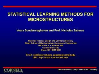
1. STATISTICAL LEARNING METHODS FOR MICROSTRUCTURES Veera Sundararaghavan and Prof. Nicholas Zabaras Materials Process Design and Control Laboratory Sibley School of Mechanical and Aerospace Engineering188 Frank H. T. Rhodes Hall Cornell University Ithaca, NY 14853-3801 Email: vs85@cornell.edu, zabaras@cornell.edu URL: http://mpdc.mae.cornell.edu/

2. WHAT IS STATISTICAL LEARNING Statistical learning is all about automating the process of searching for patterns from large scale statistics. Which patterns are interesting? Mathematical techniques for associating input data with desired attributes and identifying correlations A powerful tool for designing materials

3. FOR MICROSTRUCTURES? • Properties of a material are affected by the underlying microstructure • Microstructural attributes related to specific properties • Examples: Correlation functions -> Elastic moduli • Orientation distribution ->Yield stress in polycrystals • Attributes evolve during processing (thermo mechanical, chemical, solidification etc.) • Can we identify specific patterns in these relationships? • Is it possible to probabilistically predict the best microstructure and the best processing paths for optimizing properties based on available structural attributes?

4. TERMINOLOGY Microstructure can be represented in terms of typical attributes Examples are volume fractions, probability functions, shape/size attributes, orientation of grains, cluster functions, lineal measures and so on All these attributes affect physical properties Attributes evolve during processing of a microstructure Attributes are represented in a discrete (vector) form as ‘features’ ‘features’ are represented as a vector xk, k = 1,…,n where n is the dimensionality of the feature Every different feature is represented as xk(i) where superscript denotes the ith feature that we are interested in

5. TERMINOLOGY Given a data set of computational or experimental microstructures, can we learn the functional differences between them based on features? We denote microstructures that are similar in attributes in terms of a class representation ‘y’, y = 1..k where k is number of classes. Classes are formed into hierarchies: Each level represented by feature x(i). Structure based classes are affiliated with process and properties: powerful tool for exploring complex microstructure design space

6. APPLICATIONS

7. MICROSTRUCTURE LIBRARIES FOR REPRESENTATION Input microstructure Sundararaghavan & Zabaras, Acta Materialia, 2004 Pre-processing Identify and add new classes Feature Detection Employ lower-order features Classifier quantification and mining associations

8. MICROSTRUCTURE RECONSTRUCTION Sundararaghavan and Zabaras, Computational Materials Sci, 2005 Process Pattern recognition Microstructure evolution models 2D Imaging techniques Feature extraction Reverse engineer process parameters Database vision Microstructure Analysis (FEM/Bounding theory) 3D realizations

9. PROCESS DESIGN ALGORITHMS • 1. Exact methods • (Sensitvities) • Heuristic methods STATISTICAL LEARNING TOOLBOX Training samples NUMERICAL SIMULATION OF MATERIAL RESPONSE Update data In the library • Multi-length • scale analysis • Polycrystalline • plasticity STATISTICAL LEARNING TOOLBOX Image • Functions: • Classification methods • Identify new classes ODF Associate data with a class; update classes Process controller Pole figures

10. DESIGNING PROCESSES FOR MICROSTRUCTURES Sundararaghavan and Zabaras, Acta Materialia, 2005 DATABASE Process sequence-2 New process parameters ODF history Reduced basis Process sequence-1 Process parameters ODF history Reduced basis New dataset added Desired texture/property Classifier Adaptive basis selection Process Reduced basis Optimization Probable Process sequences & Initial parameters Stage - 1 Stage - 2 Optimum parameters Materials Process Design and Control Laboratory

11. THIS LECTURE WILL COVER…. • This lecture we will try to go into the math behind statistical learning and learn two really useful techniques – Support Vector Machines and Bayesian Clustering. • Applications to microstructure representation, reconstruction and process design will be shown • We will skim over the physics and some important computational tools behind these problems

12. Input Attributes Input Attributes Input Attributes Density Estimator Prediction of real-valued output Prediction of categorical output Probability Regressor Classifier STATISTICAL LEARNING TECHNIQUES

13. Input Attributes Input Attributes Input Attributes Density Estimator Prediction of real-valued output Prediction of categorical output Probability Regressor Classifier STATISTICAL LEARNING TECHNIQUES This lecture

14. Input Attributes Input Attributes Input Attributes Density Estimator Prediction of real-valued output Prediction of categorical output Probability Regressor Classifier STATISTICAL LEARNING TECHNIQUES This lecture Function approximation: Useful for prediction in regions that are computationally unreachable (not covered in this lecture)

15. x Classifier Microstructure features Decision Function y = w.f(x)+b Microstructure classes eg. based on a property y PRELIMINARIES OF SUPERVISED CLASSIFIERS Low strength denotes +1 denotes -1 Two class problem: The classes for the test specimens are known apriori Aim: To predict the strength of a new microstructure Pore density High strength Volume fraction

16. SUPPORT VECTOR MACHINES f(x,w,b) = sign(w. x- b) denotes +1 denotes -1 How would you classify this data?

17. OCCAM’S RAZOR plurality should not be assumed without necessity William of Ockham, Surrey (England) 1285-1347 AD, theologian • Simpler models are more likely to be correct than complex ones • Nature prefers simplicity. • principle of uncertainty maximization

18. SUPPORT VECTOR MACHINES f(x,w,b) = sign(w. x- b) denotes +1 denotes -1 How would you classify this data?

19. SUPPORT VECTOR MACHINES f(x,w,b) = sign(w. x- b) denotes +1 denotes -1 Any of these would be fine.. ..but which is best?

20. SUPPORT VECTOR MACHINES f(x,w,b) = sign(w. x- b) denotes +1 denotes -1 Define the margin of a linear classifier as the width that the boundary could be increased by before hitting a datapoint.

21. SUPPORT VECTOR MACHINES f(x,w,b) = sign(w. x- b) denotes +1 denotes -1 The maximum margin linear classifier is the linear classifier with the, um, maximum margin. This is the simplest kind of SVM (Called an LSVM) Support Vectors are those datapoints that the margin pushes up against Linear SVM

22. Plus-plane = { x : w . x + b = +1 } Minus-plane = { x : w . x + b = -1 } The vector w is perpendicular to the Plus Plane. Why? SUPPORT VECTOR MACHINES M = Margin Width x+ “Predict Class = +1” zone x- How do we compute M in terms of w and b? “Predict Class = -1” zone wx+b=1 wx+b=0 Claim: x+ = x- + lw for some value of l. Why? wx+b=-1 Let u and v be two vectors on the Plus Plane. What is w . ( u – v ) ? And so of course the vector w is also perpendicular to the Minus Plane

23. What we know: w . x+ + b = +1 w . x- + b = -1 x+ = x- + lw |x+ - x- | = M It’s now easy to get M in terms of w and b SUPPORT VECTOR MACHINES Computing the margin width M = Margin Width x+ “Predict Class = +1” zone x- “Predict Class = -1” zone wx+b=1 w . (x - + lw) + b = 1 => w . x -+ b + lw .w = 1 => -1 + lw .w = 1 => wx+b=0 wx+b=-1

24. SUPPORT VECTOR MACHINES M = “Predict Class = +1” zone wx+b=1 “Predict Class = -1” zone wx+b=0 wx+b=-1 Minimizew.w What are the constraints? w . xk + b >= 1 if yk = 1 w . xk + b <= -1 if yk = -1 Learning the Maximum Margin Classifier

25. denotes +1 denotes -1 SUPPORT VECTOR MACHINES • This is going to be a problem! • What should we do? • Minimize • w.w+ C (distance of error points to their correct place)

26. SUPPORT VECTOR MACHINES M = e11 e2 wx+b=1 e7 wx+b=0 wx+b=-1 Minimize Constraints? w . xk + b >= 1-ek if yk = 1 w . xk + b <= -1+ek if yk = -1 ek >= 0 for all k

27. x=0 SUPPORT VECTOR MACHINES What can be done about this? Harder 1-dimensional dataset

28. SUPPORT VECTOR MACHINES Quadratic Basis Functions x=0

29. SUPPORT VECTOR MACHINES WITH KERNELS Φ: x→φ(x) Minimize Constraints? w . F(xk)+ b >= 1-ek if yk = 1 w . F(xk)+ b <= -1+ek if yk = -1 ek >= 0 for all k

30. SUPPORT VECTOR MACHINES: QUADRATIC PROGRAMMING Maximize where Subject to these constraints: Then define: Datapoints with ak > 0 will be the support vectors Then classify with: f(x,w,b) = sign(w. (x)- b)

31. MULTIPLE CLASSES Given a new microstructure with its ‘s’ features given by find the class of 3D microstructure (y ) to which it is most likely to belong. • One Against One Method: • Step 1: Pair-wise classification, for a p class problem • Step 2: Given a data point, select class with maximum votes out of Materials Process Design and Control Laboratory p = 3 B Class-B C Class-A C A B A Class-C

32. Heyn int. Histogram 3D Microstructures Rose of intersections 3D Microstructures Class - 1 Class - 1 Class - 2 Class - 2 Class - 3 Class - 4 FEATURE – 1: GRAIN SHAPE FEATURE – 2 GRAIN SIZES MULTIPLE FEATURES HIERARCHICAL LIBRARIES – (a.k.a) DIVISIVE CLUSTERING

33. DYNAMIC MICROSTRUCTURE LIBRARY: CONCEPTS Space of all possible microstructures A class of microstructures (eg. equiaxial grains) New class: partition Hierarchical sub-classes (eg. medium grains) Expandable class partitions (retraining) distance measures New class Dynamic Representation: New microstructure added Axis for representation Updated representation Materials Process Design and Control Laboratory

34. QUANTIFICATION OF DIVERSE MICROSTRUCTURE A Common Framework for Quantification of Diverse Microstructure Qualitative representation Equiax grains Grain size: small Lower order descriptor approach Grain size distribution No. of grains Grain size number Equiaxial grain microstructure space Quantitative approach Microstructure represented by a set of numbers Representation space of all possible polyhedral microstructures Materials Process Design and Control Laboratory

35. BENEFITS • A data-abstraction layer for describing microstructural information. • An unbiased representation for comparing simulations and experiments AND for evaluating correlation between microstructure and properties. • A self-organizing database of valuable microstructural information which can be associated with processes and properties. • Data mining: Process sequence selection for obtaining desired properties • Identification of multiple process paths leading to the same microstructure • Adaptive selection of basis for reduced order microstructural simulations. • Hierarchical libraries for 3D microstructure reconstruction in real-time by matching multiple lower order features. • Quality control: Allows machine inspection and unambiguous quantitative specification of microstructures. Materials Process Design and Control Laboratory

36. PRINCIPAL COMPONENT ANALYSIS Let be n images. • Vectorize input images • Create an average image • Generate training images • Create correlation matrix (Lmn) • Find eigen basis (vi) of the correlation matrix • Eigen microstructures (ui) are generated from the basis (vi) as • Any new face image ( ) can be transformed to eigen face components through ‘n’ coefficients (wk) as, Reduced basis Data Points Representation coefficients Materials Process Design and Control Laboratory

37. REQUIREMENTS OF A REPRESENTATION SCHEME A set of numbers which completely represents a microstructure within its class REPRESENTATION SPACE OF A PARTICULAR MICROSTRUCTURE Must differentiate other cases: (must be statistically representative) Need for a technique that is autonomous, applicable to a variety of microstructures, computationally feasible and provides complete representation Materials Process Design and Control Laboratory

38. PCA REPRESENTATION OF MICROSTRUCTURE – AN EXAMPLE Input Microstructures Eigen-microstructures Representation coefficients (x 0.001) Basis 1 Image-1 quantified by 5 coefficients over the eigen-microstructures Basis 5 Materials Process Design and Control Laboratory

39. EIGEN VALUES AND RECONSTRUCTION OVER THE BASIS Significant eigen values capture most of the image features 4 3 2 1 Reconstruction of microstructures over fractions of the basis 1.Reconstruction with 100% basis 3. Reconstruction with 60% basis 2. Reconstruction with 80% basis 4. Reconstruction with 40% basis Materials Process Design and Control Laboratory

40. INCREMENTAL PCA METHOD • For updating the representation basis when new microstructures are added in real-time. • Basis update is based on an error measure of the reconstructed microstructure over the existing basis and the original microstructure Newly added data point Updated Basis IPCA : Given the Eigen basis for 9 microstructures, the update in the basis for the 10th microstructure is based on a PCA of 10 x 1 coefficient vectors instead of a 16384 x 1 size microstructures. Materials Process Design and Control Laboratory

41. ROSE OF INTERSECTIONS FEATURE – ALGORITHM (Saltykov, 1974) Identify intercepts of lines with grain boundaries plotted within a circular domain Total number of intercepts of lines at each angle is given as a polar plot called rose of intersections Count the number of intercepts over several lines placed at various angles. Materials Process Design and Control Laboratory

42. GRAIN SHAPE FEATURE: EXAMPLES Materials Process Design and Control Laboratory

43. GRAIN SIZE PARAMETER Several lines are superimposed on the microstructure and the intercept length of the lines with the grain boundaries are recorded (Vander Voort, 1993) The intercept length (x-axis) versus number of lines (y-axis) histogram is used as the measure of grain size. Materials Process Design and Control Laboratory

44. GRAIN SIZE FEATURE: EXAMPLES Materials Process Design and Control Laboratory

45. SVM TRAINING FORMAT GRAIN FEATURES: GIVEN AS INPUT TO SVM TRAINING ALGORITHM Data point CLASSIFICATION SUCCESS % Materials Process Design and Control Laboratory

46. CLASS HIERARCHY Level 1 : Grain shapes Class –2 Class –1 Level 2 : Subclasses based on grain sizes Class 1(a) Class 1(b) Class 1(c) Class 2(a) Class 2(b) Class 2(c) New classes: Distance of image feature from the average feature vector of a class Materials Process Design and Control Laboratory

47. IPCA QUANTIFICATION WITHIN CLASSES Class-j Microstructures (Equiaxial grains, medium grain size) Class-i Microstructures (Elongated 45 degrees, small grain size) The Library – Quantification and image representation Materials Process Design and Control Laboratory

48. REPRESENTATION FORMAT FOR MICROSTRUCTURE Date: 1/12 02:23PM, Basis updated Shape Class: 3, (Oriented 40 degrees, elongated) Size Class : 1, (Large grains) Coefficients in the basis:[2.42, 12.35, -4.14, 1.95, 1.96, -1.25] Improvement of microstructure representation due to classification Reconstruction with 6 coefficients (24% basis): A class with 25 images Improvement in reconstruction: 6 coefficients (10 % of basis) Class of 60 images Original image Reconstruction over 15 coefficients Materials Process Design and Control Laboratory

49. MICROSTRUCTURE REPRESENTATION USING SVM & PCA Materials Process Design and Control Laboratory • A DYNAMIC LIBRARY APPROACH • Classify microstructures based on lower order descriptors. • Create a common basis for representing images in each class at the last level in the class hierarchy. • Represent 3D microstructures as coefficients over a reduced basis in the base classes. • Dynamically update the basis and the representation for new microstructures Does not decay to zero COMMON-BASIS FOR MICROSTRUCTURE REPRESENTATION

50. PCA MICROSTRUCTURE RECONSTRUCTION Materials Process Design and Control Laboratory Basis Components Reconstruct using two basis components X5.89 + X14.86 Project onto basis Pixel value round-off Representation using just 2 coefficients (5.89,14.86)