Download
1 / 32
330 likes | 512 Vues
Step three: statistical analyses to test biological hypotheses. General protocol continued. Biological hypotheses and statistical tests. Hypotheses driven by Biology Statistics depend on data and hypotheses NO NEW STATISTICAL TOOLS ARE NEEDED FOR MORPHOMETRICS!!

E N D
Step three: statistical analyses to test biological hypotheses General protocol continued
Biological hypotheses and statistical tests • Hypotheses driven by Biology • Statistics depend on data and hypotheses • NO NEW STATISTICAL TOOLS ARE NEEDED FOR MORPHOMETRICS!! • Explanatory hypotheses: relative position of specimens in data space:relationship among specimens in data space • Confirmatory hypotheses: compare groups, associate shape with other variables, etc.
Some hypotheses (shape related) • How do populations and species differ? • Does the observed variation generate a predictable pattern? • Are there additional factors (ecological, evolutionary) correlated with variation? • How does shared evolutionary history affect the observed patterns?
Do populations differ? Is there a predictable pattern? Correlated factors? Effect of phylogeny? MANOVA, CVA PCA, UPGMA Regression, 2B-PLS Comparative Method Hypotheses as statistical tests
Exploratory data analysis • Investigate data using only Y-matrix of shape variables (PWScores + U1,U2) • Specimens are points in high-dimensional data space • Look for patterns and distributions of points • Generate summary plot of data space (ordination) • Look for relationships of points (clustering)
Ordination and dimension reduction • Visualize high dimensional data space as succinctly as possible • Describe variation in original data with new set of variables (typically orthogonal vectors) • Order new variables by variation explained (most – least) • Plot first few dimensions to summarize data • Principal Components Analysis (PCA) one approach (others include: PCoA, MDS, CA, etc.)
PCA: what does it do? • Rotates data so that main axis of variation (PC1) is horizontal • Subsequent PC axes are orthogonal to PC1, and are ordered to explain sequentially less variation • The goal is to explain more variation in fewer dimensions
PCA: interpretations • Eigenvectors are linear combinations of original variables (interpreted by PC loadings of each variable) • PCA PRESERVES EUCLIDEAN DISTANCES among objects • PCA does NOTHING to the data, except rotate it to axes expressing the most variation; it loses NO INFORMATION (if all PC vectors retained) • If the original variables are uncorrelated, PCA not helpful in reducing dimensionality of data • PCA does not find a particular factor (e.g., group differences, allometry): it identifies the direction of most variation, which may be interpretable as a ‘factor’ (but may not)
Clustering • Data are dots in a high-dimensional space (Y-matrix) • Can we connect to dots for groupings, where clusters represent groups of similar specimens? • Cluster methods generate ‘1-dimensional view’ of relationships, based on some criterion • Clustering requires distance (or similarity) between points • MANY different criteria • Clustering is algorithmic, not algebraic (i.e., it is a procedure, or set of rules for connecting data)
Conclusions: exploratory methods • Useful tools for summarizing shape variation • Help you understand your data through visualizing variation (both ordination plots and cluster diagrams) • Help describe relationships among specimens in terms of overall similarity
Confirmatory data analysis • Investigate data using shape variables (Y-matrix) and other (independent) variables (X-matrix) • Test for patterns of shape variation • Independent variables determine type of statistical test
Types of independent variables • Categorical: variables delineating groups of specimens (e.g., male/female, species, etc.) • Continuous: variables on a continuous scale (e.g., size, moisture, age, etc.) • Different statistical methods for each
Categorical: shape differences among groups Continuous: relationship of variables and shape Continuous: association of variables and shape MANOVA Mult. Regression 2B-PLS (2-Block Partial Least squares) Some statistical tests MANOVA and multivariate regression are both GLM statistics (General Linear Models)
Group differences: MANOVA • Is there a difference in shape between groups? • Multivariate generalization of ANOVA • Compares variation within groups to variation between groups • Significant MANOVA: Group means are different in shape
MANOVA • RW1-RW30 Utah chub • Source Sex Loc Sex X loc IL/SL Size Wilks' Lambda 0.38888016 4.66 30 89 <.0001 Wilks' Lambda 0.00308619 3.26 240 706.35 <.0001 Wilks' Lambda 0.10138762 1.40 180 533.33 0.0020 Wilks' Lambda 0.61907356 1.83 30 89 0.0159 Wilks' Lambda 0.75516916 0.96 30 89 0.5318
MANOVA: post hoc tests • Pairwise comparisons using Generalized Mahalanobis Distance (D2 or D) • Convert D2→T2 → F to test • For experiment-wise error rate, adjust using Bonferroni: α exp = α / # comparisons
Discriminant analysis: CVA & DFA • ‘Combination’ of MANOVA and PCA • Tests for group differences (MANOVA) • PCA of among-group variation relative to within-group variation • Suggests which groups differ on which variables • Can ‘classify’ specimens to groups • Special case: 2 groups= discriminant function analysis (DFA)
DFA/CVA: post-hoc tests • For DFA/CVA, compare difference among groups using Generalized Mahalanobis Distance (D2) • Mahalanobis D2 is logical choice because CVA/DFA is MANOVA, and the PCA is relative to within-group variability (i.e., VCV ‘standardized’) • Convert D2→T2 → F to perform statistical test • Experiment-wise error rate adjusted as before (i.e., adjusted α)
Continuous variation: regression • Is there a relationship between shape and some other variable? • Multivariate regression of shape on continuous variable • Significant regression implies shape changes as a function of other variable (e.g., size)
Example of shape on size in mountain sucker Multivariate tests of significance: Statistic Value Fs df1 df2 Prob Wilks' Lambda: 0.34356565 22.822 36 430.0 3.580E-078 Pillai's trace: 0.65643435 22.822 36 430.0 3.580E-078 Hotelling-Lawley trace: 1.91065190 22.822 36 430.0 3.580E-078 Roy's maximum root: 1.91065190 22.822 36 430.0 3.580E-078 Test that kth root and those that follow are zero: k U Fs df1 df2 Prob 1 0.34356565 22.822 36 430.0 3.580E-078
Continuous variation: association 2B-PLS • Is there an association between shape and some other set of variables (not causal)? • Find pairs of linear combinations for X & Y that maximize the covariation between data sets • Linear combinations are constrained to be orthogonal within each set (like PC axes) but NOT between data sets • Calculations less complicated for 2B-PLS (because fewer mathematical constraints) • Analogous to ‘multivariate correlation’ • 2B-PLS is called SINGULAR WARPS when shape is one or more of the data sets. Bookstein et al., 2003: J. of Hum. Evol.)
Resampling methods • Methods that take many samples from original data set in some specified way and evaluate the significance of the original based on these samples • Resampling approaches are nonparametric, because they do not depend of theoretical distributions for significance testing (they generate a distribution from the data) • Are very flexible, and can allow for complicated designs • Very useful in morphometrics, and can be used for: • Testing standard designs • Testing non-standard designs • Testing when sample sizes small relative to # of variables
Randomization (permutation) • Proposed by Fisher (1935) for assessing significance of 2-sample comparison (Fisher’s exact test) • Fisher’s exact test: a total enumeration of possible pairings of data • Randomization can be used to determine most any test statistic • Protocol • Calculate observed statistic (e.g., T-statistic): Eobs • Reorder data set (i.e. randomly shuffle data) and recalculate statistic Erand • Repeat many times to generate distribution of statistic • Percentage of Erand more extreme than Eobs is significance level
Randomization: comments • Randomization EXTREMELY useful and flexible technique • How and what to resample depends upon data and hypothesis • Regression and correlation: shuffle Y vs. X • Group comparison (e.g., ANOVA): shuffle Y on groups • Some tests (e.g., t-test) may depend on direction (1-tailed vs. 2-tailed) • Also useful when no theoretical distribution exists for statistic, or when design is ‘non-standard’ • This is frequently the case in E&E studies
Step four: Graphical depiction of results • Strength of landmark-based TPS approach • Can view deformation of TPS grid among groups or with continuous variable
Effect of relative intestinal length: measure of trophic level Long IL/SL 3.0 Short IL/SL 0.72