Download
1 / 23
230 likes | 361 Vues
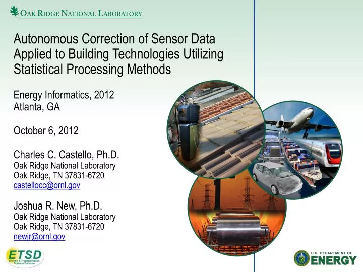
Autonomous Correction of Sensor Data Applied to Building Technologies Utilizing Statistical Processing Methods Energy Informatics, 2012 Atlanta, GA October 6, 2012 Charles C. Castello, Ph.D. Oak Ridge National Laboratory Oak Ridge, TN 37831-6720 castellocc@ornl.gov Joshua R. New, Ph.D.

E N D
Autonomous Correction of Sensor Data Applied to Building Technologies Utilizing Statistical Processing Methods Energy Informatics, 2012 Atlanta, GA October 6, 2012 Charles C. Castello, Ph.D. Oak Ridge National Laboratory Oak Ridge, TN 37831-6720 castellocc@ornl.gov Joshua R. New, Ph.D. Oak Ridge National Laboratory Oak Ridge, TN 37831-6720 newjr@ornl.gov
Table of Contents • Background • Challenges • Methods • Statistical Techniques • Example • Experimental Dataset • Results • Best Performers • Summary • Future Work
Background • Energy consumption in the U.S. is a critical area of concern where residential and commercial buildings consume approximately 40% of total primary energy. • Retrofitting inefficient existing buildings with new and innovative technologies that help to curb energy consumption. • Standing seam metal roofs that exploit infrared-reflective paint pigments to boost solar reflectance • Pella® triple-pane, low emittance, Argon filled windows • ClimateMaster ®’s high-efficiency, water-to-air heat pump for space conditioning • ClimateMaster ®’s high-efficiency, water-to-water heat pump for hot water heating • Fantech Energy Recovery Ventilator (ERV) which replaces air inside of a home with fresh air
Research in Energy Efficiency • There is much research dealing with the improvement of energy efficiency in commercial buildings and residential homes. • This research includes several fundamental concerns relevant to sensors being used to collect a wide variety of variables. • Concerns include: • Accuracy • Performance • Reliability • Variables include: • Temperature • Time • Wind speed
ZEBRAlliance Project • Sensors are an imperative tool in analyzing these technologies and determining their impact. • Example of this is ORNL’s ZEBRAllianceProject which consists of 4 homes: • 1st home 279 sensors • 2nd home 279 sensors • 3rd home 321 sensors • 4th home 339 sensors The majority of these sensors are temperature, humidity, pressure, and energy. Home #2 Home #4 Home #3 Home #1
More on the ZEBRAlliance Project • The ZEBRAlliance Project broke ground on September 26, 2008. • Research project and multi-faceted educational campaign to influence consumers that energy efficient homes can be: • Real • Desirable • Affordable • Located in the Crossroads at Wolf Creek Subdivision in Oak Ridge, TN. • Energy savings of approximately 55-60% compared with traditional new construction. • Data is being collected for a span of three years. • After the research period has ended, all four homes will be sold.
Dealing with Large Amounts of Data • Most sensors have a 15-minute resolution for ORNL’s ZEBRAlliance project with approximately 80 sensors having a 1-minute resolution: • 9,352 data points in an hour • 224,448 in a day • 1,571,136 in a week • 81,699,072 in a year • Many issues arise with this amount of data points being collected in such a real-world experiment, specifically data corruption from: • Sensor failing to produce data. • Fouling of the sensor’s interface due to the environment which produces inaccurate data. • A sensor’s calibration being incorrect, producing inaccurate data. • Data logger failure which causes missing data.
Current Data Validation Methods • There are currently two approaches that are widely used for validation of data: • Analytical redundancy • Hardware redundancy • Analytical redundancy uses data from multiple sensors to predict a sensor’s value. • An example is using a temperature and humidity channel to predict heat flux. • When the number of sensors increases, the complexity of the model increases. • Hardware redundancy is not always possible due to the need for increased amount of resources: • Sensors • Data acquisition
Sensor Validation Techniques • Sensor data validation techniques are needed that minimizes the amount of needed resources: • Hardware • Software • Sensor data validation techniques are also required to be: • Automated • Able to handle large amounts of data • Able to handle different types of data • Correct missing and corrupt data • Data collected through ORNL’s ZEBRAlliance project has a maximum error rate of 14.59% (per month) for data logger and sensor failure (does not include sensor fouling and calibration error).
Effects of Inaccurate Data • Data collected by sensors in residential buildings are not only used to determine the impact of energy efficiency technologies but also used for: • Control • Modeling • An example of the influence inaccurate data has on models, Nonhebel 1994 did a study of using inaccurate data to predict crop growth. • Using inaccurate data caused deviations up to 30% in simulated yields. • Studies have not been done on the influence inaccurate data has on building applications. • Using the figure in the previous slide, imagine a 14.59% deviation in cost or simple payback for investing in an energy efficiency technology for your home. This inaccuracy is substantial!
Statistical Processing Methods • Statistical methods from Bo et al., 2009 were used to predict wireless field strength: • Least squares • Maximum likelihood estimation • Segmentation averaging • Threshold based • Modified to meet the needs of fault detection and sensor data prediction for building applications. • Artificial gaps are introduced into the dataset by randomly removing portions of existing data for testing the accuracy of auto-correcting algorithms. • Accomplished by randomly generating training and testing subsets: • Training set represents 70% of original dataset. • Testing set represents 30% of original dataset.
Predict Missing Data • Each sensor is used as an independent variable and predicts sensor values based upon a variable-sized window of observations. • A prediction model is generated for each window of observations and correction occurs if values are missing or corrupt: • Interpolation • Extrapolation • An observation window of size wis used to predict the sensor’s data value for each time-step within the observation window. • The observation window moves forward by wtime-steps (no overlap) and prediction for each sample within the observation window is calculated. • Actual value vs. predicted value is measured: • Root-mean-square error (RMSE) • Relative error • Absolute error
Example of Missing Data • Let’s say we have 18 samples of temperature data with a 15-minute resolution (4 ½ hours). • However, a chunk of data is missing. • How do we correct this? • Generate a model based on data that we have obtained. • Interpolate based on that model for missing data values. Missing Data
Example of Predicting Data • Least squares method is used with 15-minute temperature data with an observation window of size w=24. • Data is split into training (70%) and testing (30%) subsets. • During training, each observation window generates a model based on the training samples in that window. • The model is used to predict the behavior of temperature in that observation window. * Based on 10th observation window.
What is an observation window? • Let’s say we have a observation window size of w=2 with 15-minute temperature data for 3 hours. • That gives us 12 data points; (N=12) (w=2) = 6 observation windows. • We must generate a prediction model for each observation window using the training data. • Then use this model to predict where the testing data points are located. 15-minute data for 3 hours
Performance Metrics • Root-mean-square error (RMSE): • where: • r is the residual value between the actual and predicted data • Relative error: • where: • n is the current time-step • s represents the first time-step of the observation window • y(s) is the actual sensor data • r(s) is the residual corresponding to y(s) • Absolute error: • where: • ymax and ymin are the maximum and minimum sensor data values respectively of the sensor dataset, Y
Experimental Dataset • Taken from ORNL’s ZEBRAlliance project, specifically: • Temperature (°F) “Z09_T_ERV_IN_Avg” Temperature of ERV intake from outside • Humidity (%RH) “Z09_RH_ERVin_Avg” Humidity of ERV intake from outside • Energy usage (Wh) “A01_WH_fridge_tot” Energy of refrigerator • Data collected using Campbell Scientific’s CR1000 data logger. • There are four homes in the ZEBRAlliance project. • Data was taken from the 2nd home • During the 2010 calendar year (N=35,040) • Technologies in home #2 • Advanced framing • High-efficiency florescent lighting • Energy Star appliances • Water-to-air heat pumps (WAHP) • Water-to-water heat pumps (WWHP)
Best Performers (Temperature Data) Observation Window Sizes • w=6 (1 ½ hours) • w=12 (3 hours) • w=24 (6 hours) • w=48 (1/2 day) • w=96 (1 day) * RMSE – Root-mean-square error ** RE – Relative error *** AE – Absolute error
Best Performers (Humidity Data) Observation Window Sizes • w=6 (1 ½ hours) • w=12 (3 hours) • w=24 (6 hours) • w=48 (1/2 day) • w=96 (1 day) * RMSE – Root-mean-square error ** RE – Relative error *** AE – Absolute error
Best Performers (Energy Data) Observation Window Sizes • w=6 (1 ½ hours) • w=12 (3 hours) • w=24 (6 hours) • w=48 (1/2 day) • w=96 (1 day) * RMSE – Root-mean-square error ** RE – Relative error *** AE – Absolute error
Summary • Four statistical processing methods are used to validate temperature, humidity, and energy data in residential buildings for autonomous detection and correction of missing or corrupt sensor data. • Least squares • Maximum likelihood estimation • Segmentation averaging • Threshold based • Independent data validation is accomplished using observation windows (i.e., subset of samples) with wobservations to build a model of the data. • Data validation and correction occurs for each successive observation window within the sensor dataset using interpolation and/or extrapolation for missing and corrupt data.
Summary • Results • The threshold based technique performed best with: • Temperature (c=2) • Humidity (c=2) • Energy data (c=1) • It is anticipated that temperature, relative humidity, and energy data would follow similar patterns in other buildings, but additional studies are needed to confirm the degree to which these results generalize across other buildings. • Other Future Research Work • Studying other types of methods besides statistical such as: • Filtering • Machine learning • Other data types will also be investigated: • Heat flux • Airflow • Liquid flow