Construction and Evaluation of Response Surface Designs Incorporating Bias from Model Misspecification

1. Construction and Evaluation of Response Surface Designs Incorporating Bias from Model Misspecification Connie M. Borror, Arizona State University West Christine M. Anderson-Cook, Los Alamos National Laboratory Bradley Jones, JMP SAS Institute

2. Motivation • Response surface design evaluation (and creation) assuming a particular model • Single number efficiencies • Prediction variance performance • Mean-squared error • Model misspecification? • What effect does this have on prediction and optimization?

3. Motivation • Examine effect of model misspecification • Expected squared bias • Prediction variance • Expected mean squared error • Using fraction of design space (FDS) plots and box plots • Evaluate designs based on the contribution of ESB relative to PV.

4. Scenario • Cuboidal regions • True form of the model is of higher order than the model being fit. • Examine • Response surface models when the true form is cubic • Screening experiment when the true form is full second order.

5. Model Specifications • The model to be fit is Y = X11 + ε • X1 = n × p design matrix for the assumed form of the model • The true form of the model is Y = X11+ X22 + ε • X2 = n × q design matrix pertaining to those parameters (2) not present in the model to be fit (assumed model).

6. Model Specifications • 2in general, are not fully estimable • Assume 2~ N(0, )

7. Criteria • Mean-squared error • Expected squared bias (ESB): • Expected MSE sum of PV and ESB

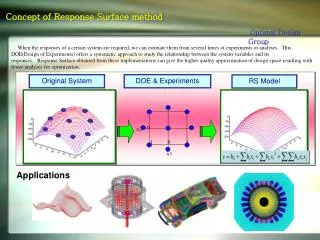
8. Fraction of Design Space (FDS) Plots • Zahran, Anderson-Cook, and Myers (2003) scaled prediction variance values are plotted versus the fraction of the design space that has SPV at or below the given value • Adapt this to plot ESB and EMSE as well as PV. • We use FDS plots and box plots to assess the designs

9. Cases • I. Two-factor response surface design • Assume a second-order model: • True form of the model is cubic:

10. Case I Designs • Central Composite Design (CCD) • Quadratic I-optimal (Q I-opt) • Quadratic D-optimal (Q D-opt) • Cubic I-optimal (C I-opt) • Cubic D-optimal (C D-opt) • Cubic Bayes I-optimal (C Bayes I-opt) • Cubic Bayes D-optimal (C Bayes D-opt)

11. Case I • CCD

12. Case I Designs • CCD (ESB and EMSE performance as bias increases)

13. Case I Designs • PV for all designs

14. Case I Designs • ESB for all designs

15. Case I Designs • EMSE for all designs

16. Case I Designs • FDS for EMSE for all designs

17. Case II • Four factor response surface design • Assume a second-order model: • True form of the model is cubic: • 20 additional terms as we move from the second-order model to cubic.

18. Case II Designs • Six possible designs, with n = 27 runs • Central Composite Design (CCD) • Box Behnken Design (BBD) • Quadratic I-optimal (Q I-Opt) • Quadratic D-optimal (Q D-Opt) • Cubic Bayes I-optimal (C Bayes I-Opt) • Cubic Bayes D-optimal (C Bayes D-Opt) Note: Cubic I- and D-Optimal not possible with available size of design

19. Case II • PV for all designs

20. Case II • EMSE for all designs

21. Case II FDS plot of EMSE for Four Factors

22. Case III • Eight-factor Screening Design • Assume a first-order model: • True form of the model is full second-order:

23. Case III Designs • 28-4 fractional factorial design with 4 center runs • D-optimal (for first order) • Bayes I-optimal (for second order) • Bayes D-optimal (for second order)

24. Case III Designs • The difference in the number of terms from the assumed to the true form of the models increases from 8 to 44. • We would expect bias to quickly dominate EMSE.

25. Case III • PV for all designs

26. Case III • ESB for all designs

27. Case III • EMSE for all designs

28. Design Notes • For the two-factor case: • The I-optimal and CCD were equivalent. • They performed the best based on minimizing the maximum EMSE • They performed the best based on prediction variance

29. Design Notes • For the four factor case, • the BBD was best based on EMSE criteria (in particular, the 95th percentile, median, mean) • when size of the coefficients of missing terms are moderate to large • The I-optimal design was competitive for this case only if small amounts of bias were present. • As the number of missing cubic terms increases, the BBD was best for EMSE.

30. Design Notes • I-optimal designs were highly competitive over 95% of the design region; not with respect to the maximum PV, ESB, and EMSE. • Cubic Bayesian designs did not perform well.

31. Design Notes • In the screening design example: • The D-optimal designs best if the assumed model is correct, but break down quickly if quadratic terms are in the model • Much more pronounced than in the response surface design cases. • Quadratic Bayesian I-optimal design was best based on mean, median, and 95th percentile of EMSE • The 28-4 fractional factorial design was best with respect to the maximum EMSE. • The 28-4 design was best for both PV and ESB when the PV and ESB contribution to the model were balanced.

32. Conclusions • Appropriate design can strongly depend on the assumption that we know the true form of the underlying model • If we select designs carefully it is often possible to select a model that predicts well in the design space, and provide some protection against missing model terms. • The ESB approach to assessing the effect of missing terms provides is advantageous: • do not have to specify coefficient values for the true underlying model, • Instead, the relative size of the missing terms can be calibrated relative to the variance of the observations.

33. Conclusions • Size of the bias variance relative to observational error needed to balance contributions from PV and ESB is highly dependent on the number of missing terms from the assumed model. • As the number of missing terms increases, the ability of designs to cope with the bias decreases substantially • different designs are able to handle this increasing bias differently.