View on Cold in 17 th Century

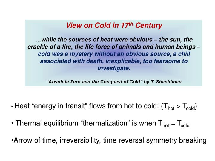
1. View on Cold in 17th Century …while the sources of heat were obvious – the sun, the crackle of a fire, the life force of animals and human beings – cold was a mystery without an obvious source, a chill associated with death, inexplicable, too fearsome to investigate. “Absolute Zero and the Conquest of Cold” by T. Shachtman • Heat “energy in transit” flows from hot to cold: (Thot > Tcold) • Thermal equilibrium “thermalization” is when Thot = Tcold • Arrow of time, irreversibility, time reversal symmetry breaking

2. Zeroth law of thermodynamics If two systems are separately in thermal equilibrium with a third system, they are in thermal equilibrium with each other. A C Diathermal wall C can be considered the thermometer. If C is at a certain temperature then A and B are also at the same temperature. B C

4. Simplified constant-volume gas thermometer Pressure (P = gh) is the thermometric property that changes with temperature and is easily measured.

5. Temperature scales • Assign arbitrary numbers to two convenient temperatures such as melting and boiling points of water. 0 and 100 for the celsius scale. • Take a certain property of a material and say that it varies linearly with temperature. • X = aT + b • For a gas thermometer: • P = aT + b

6. Gas Pressure Thermometer Ice point Steam point LN2

7. Gas Pressure Thermometer Ice point Steam point LN2 Celsius scale P = a[T(oC) + 273.15]

9. Phase diagram of water Near triple point can have ice, water, or vapor on making arbitrarily small changes in pressure and temperature.

11. Concept of Absolute Zero (1703) Guillaume Amonton first derived mathematically the idea of absolute zerobased on Boyle-Mariotte’s law in 1703. For a fixed amount of gas in a fixed volume, p = kT Amonton’s absolute zero ≈ 33 K

12. Other Types of Thermometer • Metal resistor : R = aT + b • Semiconductor : logR = a-blogT • Thermocouple : E = aT + bT2 Low Temperature Thermometry

13. Platinum resistance thermometer

14. CERNOX thermometer

15. International Temperature Scale of 1990

17. 16 different configurations (microstates), 5 different macrostates

19. Microcanonical ensemble: • Total system ‘1+2’ contains 20 energy quanta and 100 levels. • Subsystem ‘1’ containing 60 levels with total energy x is in equilibrium with subsystem ‘2’ containing 40 levels with total energy 20-x. • At equilibrium (max), x=12 energy quanta in ‘1’ and 8 energy quanta in ‘2’

21. Ensemble: All the parts of a thing taken together, so that each part is considered only in relation to the whole.

22. The most likely macrostate the system will find itself in is the one with the maximum number of microstates. E2 2(E2) E1 1(E1)

23. Most likely macrostate the system will find itself in is the one with the maximum number of microstates. (50h for 100 tosses) Number of Microstates () Macrostate

24. E (E) Microcanonical ensemble: An ensemble of snapshots of a system with the same N, V, and E A collection of systems that each have the same fixed energy.

25. Canonical ensemble: An ensemble of snapshots of a system with the same N, V, and T (red box with energy  << E. Exchange of energy with reservoir. E- (E-)  I()

26. 1 1 1 1 1 1 1 1 1 1 1 1 1 1 1 1 1 1 1 1 1 1 1 1 1 1 1 1 1 1 1 1 1 1 1 1 1 1 1 1 1 1 1 1 1 1 1 1 1 1 1 1 1 1 1 1 1 1 1 1 1 1 1 1 1 1 1 1 1 1 1 1 1 1 1 1 1 1 1 1 1 1 1 1 1 1 1 1 1 1 1 1 1 1 1 1 1 1 1 1 1 1 1 1 1 1 1 1 1 1 1

28. Canonical ensemble: P()  (E-)1  exp[-/kBT] Log10 (P()) • Total system ‘1+2’ contains 20 energy quanta and 100 levels. • x-axis is # of energy quanta in subsystem ‘1’ in equilibrium with ‘2’ • y-axis is log10 of corresponding multiplicity of reservoir ‘2’