Download
1 / 82
1.08k likes | 1.86k Vues
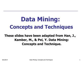
Data Mining: Concepts and Techniques — Slides for Textbook — — Chapter 6 —. © Jiawei Han and Micheline Kamber Intelligent Database Systems Research Lab School of Computing Science Simon Fraser University, Canada http://www.cs.sfu.ca. Chapter 6: Mining Association Rules in Large Databases.

E N D
Data Mining: Concepts and Techniques— Slides for Textbook — — Chapter 6 — ©Jiawei Han and Micheline Kamber Intelligent Database Systems Research Lab School of Computing Science Simon Fraser University, Canada http://www.cs.sfu.ca Data Mining: Concepts and Techniques
Chapter 6: Mining Association Rules in Large Databases • Association rule mining • Mining single-dimensional Boolean association rules from transactional databases • Mining multilevel association rules from transactional databases • Mining multidimensional association rules from transactional databases and data warehouse • From association mining to correlation analysis • Constraint-based association mining • Summary Data Mining: Concepts and Techniques
What Is Association Mining? • Association rule mining: • Finding frequent patterns, associations, correlations, or causal structures among sets of items or objects in transaction databases, relational databases, and other information repositories. • Applications: • Basket data analysis, cross-marketing, catalog design, loss-leader analysis, clustering, classification, etc. • Examples. • Rule form: “Body ® Head [support, confidence]”. • buys(x, “diapers”) ® buys(x, “beers”) [0.5%, 60%] • major(x, “CS”) ^ takes(x, “DB”) ® grade(x, “A”) [1%, 75%] Data Mining: Concepts and Techniques
Association Rule: Basic Concepts • Given: (1) database of transactions, (2) each transaction is a list of items (purchased by a customer in a visit) • Find: all rules that correlate the presence of one set of items with that of another set of items • E.g., 98% of people who purchase tires and auto accessories also get automotive services done • Applications • * Maintenance Agreement (What the store should do to boost Maintenance Agreement sales) • Home Electronics * (What other products should the store stocks up?) • Attached mailing in direct marketing • Detecting “ping-pong”ing of patients, faulty “collisions” Data Mining: Concepts and Techniques
Rule Measures: Support and Confidence Customer buys both Customer buys diaper • Find all the rules X & Y Z with minimum confidence and support • support,s, probability that a transaction contains {X Y Z} • confidence,c,conditional probability that a transaction having {X Y} also contains Z Customer buys beer Let minimum support 50%, and minimum confidence 50%, we have • A C (50%, 66.6%) • C A (50%, 100%) Data Mining: Concepts and Techniques
Association Rule Mining: A Road Map • Boolean vs. quantitative associations (Based on the types of values handled) • buys(x, “SQLServer”) ^ buys(x, “DMBook”) ® buys(x, “DBMiner”) [0.2%, 60%] • age(x, “30..39”) ^ income(x, “42..48K”) ® buys(x, “PC”) [1%, 75%] • Single dimension vs. multiple dimensional associations (see ex. Above) • Single level vs. multiple-level analysis • What brands of beers are associated with what brands of diapers? • Various extensions • Correlation, causality analysis • Association does not necessarily imply correlation or causality • Maxpatterns and closed itemsets • Constraints enforced • E.g., small sales (sum < 100) trigger big buys (sum > 1,000)? Data Mining: Concepts and Techniques
Chapter 6: Mining Association Rules in Large Databases • Association rule mining • Mining single-dimensional Boolean association rules from transactional databases • Mining multilevel association rules from transactional databases • Mining multidimensional association rules from transactional databases and data warehouse • From association mining to correlation analysis • Constraint-based association mining • Summary Data Mining: Concepts and Techniques
Mining Association Rules—An Example Min. support 50% Min. confidence 50% For rule AC: support = support({AC}) = 50% confidence = support({AC})/support({A}) = 66.6% The Apriori principle: Any subset of a frequent itemset must be frequent Data Mining: Concepts and Techniques
Mining Frequent Itemsets: the Key Step • Find the frequent itemsets: the sets of items that have minimum support • A subset of a frequent itemset must also be a frequent itemset • i.e., if {AB} isa frequent itemset, both {A} and {B} should be a frequent itemset • Iteratively find frequent itemsets with cardinality from 1 to k (k-itemset) • Use the frequent itemsets to generate association rules. Data Mining: Concepts and Techniques
The Apriori Algorithm • Join Step: Ckis generated by joining Lk-1with itself • Prune Step: Any (k-1)-itemset that is not frequent cannot be a subset of a frequent k-itemset • Pseudo-code: Ck: Candidate itemset of size k Lk : frequent itemset of size k L1 = {frequent items}; for(k = 1; Lk !=; k++) do begin Ck+1 = candidates generated from Lk; for each transaction t in database do increment the count of all candidates in Ck+1 that are contained in t Lk+1 = candidates in Ck+1 with min_support end returnkLk; Data Mining: Concepts and Techniques
The Apriori Algorithm — Example Database D L1 C1 Scan D C2 C2 L2 Scan D L3 C3 Scan D Data Mining: Concepts and Techniques
How to Generate Candidates? • Suppose the items in Lk-1 are listed in an order • Step 1: self-joining Lk-1 insert intoCk select p.item1, p.item2, …, p.itemk-1, q.itemk-1 from Lk-1 p, Lk-1 q where p.item1=q.item1, …, p.itemk-2=q.itemk-2, p.itemk-1 < q.itemk-1 • Step 2: pruning forall itemsets c in Ckdo forall (k-1)-subsets s of c do if (s is not in Lk-1) then delete c from Ck Data Mining: Concepts and Techniques
How to Count Supports of Candidates? • Why counting supports of candidates a problem? • The total number of candidates can be very huge • One transaction may contain many candidates • Method: • Candidate itemsets are stored in a hash-tree • Leaf node of hash-tree contains a list of itemsets and counts • Interior node contains a hash table • Subset function: finds all the candidates contained in a transaction Data Mining: Concepts and Techniques
Example of Generating Candidates • L3={abc, abd, acd, ace, bcd} • Self-joining: L3*L3 • abcd from abc and abd • acde from acd and ace • Pruning: • acde is removed because ade is not in L3 • C4={abcd} Data Mining: Concepts and Techniques
Methods to Improve Apriori’s Efficiency • Hash-based itemset counting: A k-itemset whose corresponding hashing bucket count is below the threshold cannot be frequent • Transaction reduction: A transaction that does not contain any frequent k-itemset is useless in subsequent scans • Partitioning: Any itemset that is potentially frequent in DB must be frequent in at least one of the partitions of DB • Sampling: mining on a subset of given data, lower support threshold + a method to determine the completeness • Dynamic itemset counting: add new candidate itemsets only when all of their subsets are estimated to be frequent Data Mining: Concepts and Techniques
Is Apriori Fast Enough? — Performance Bottlenecks • The core of the Apriori algorithm: • Use frequent (k – 1)-itemsets to generate candidate frequent k-itemsets • Use database scan and pattern matching to collect counts for the candidate itemsets • The bottleneck of Apriori: candidate generation • Huge candidate sets: • 104 frequent 1-itemset will generate 107 candidate 2-itemsets • To discover a frequent pattern of size 100, e.g., {a1, a2, …, a100}, one needs to generate 2100 1030 candidates. • Multiple scans of database: • Needs (n +1 ) scans, n is the length of the longest pattern Data Mining: Concepts and Techniques
Mining Frequent Patterns Without Candidate Generation • Compress a large database into a compact, Frequent-Pattern tree (FP-tree) structure • highly condensed, but complete for frequent pattern mining • avoid costly database scans • Develop an efficient, FP-tree-based frequent pattern mining method • A divide-and-conquer methodology: decompose mining tasks into smaller ones • Avoid candidate generation: sub-database test only! Data Mining: Concepts and Techniques
{} Header Table Item frequency head f 4 c 4 a 3 b 3 m 3 p 3 f:4 c:1 c:3 b:1 b:1 a:3 p:1 m:2 b:1 p:2 m:1 Construct FP-tree from a Transaction DB TID Items bought (ordered) frequent items 100 {f, a, c, d, g, i, m, p}{f, c, a, m, p} 200 {a, b, c, f, l, m, o}{f, c, a, b, m} 300 {b, f, h, j, o}{f, b} 400 {b, c, k, s, p}{c, b, p} 500{a, f, c, e, l, p, m, n}{f, c, a, m, p} min_support = 0.5 • Steps: • Scan DB once, find frequent 1-itemset (single item pattern) • Order frequent items in frequency descending order • Scan DB again, construct FP-tree Data Mining: Concepts and Techniques
Benefits of the FP-tree Structure • Completeness: • never breaks a long pattern of any transaction • preserves complete information for frequent pattern mining • Compactness • reduce irrelevant information—infrequent items are gone • frequency descending ordering: more frequent items are more likely to be shared • never be larger than the original database (if not count node-links and counts) • Example: For Connect-4 DB, compression ratio could be over 100 Data Mining: Concepts and Techniques
Mining Frequent Patterns Using FP-tree • General idea (divide-and-conquer) • Recursively grow frequent pattern path using the FP-tree • Method • For each item, construct its conditional pattern-base, and then its conditional FP-tree • Repeat the process on each newly created conditional FP-tree • Until the resulting FP-tree is empty, or it contains only one path(single path will generate all the combinations of its sub-paths, each of which is a frequent pattern) Data Mining: Concepts and Techniques
Major Steps to Mine FP-tree • Construct conditional pattern base for each node in the FP-tree • Construct conditional FP-tree from each conditional pattern-base • Recursively mine conditional FP-trees and grow frequent patterns obtained so far • If the conditional FP-tree contains a single path, simply enumerate all the patterns Data Mining: Concepts and Techniques
Header Table Item frequency head f 4 c 4 a 3 b 3 m 3 p 3 {} f:4 c:1 c:3 b:1 b:1 a:3 p:1 m:2 b:1 p:2 m:1 Step 1: From FP-tree to Conditional Pattern Base • Starting at the frequent header table in the FP-tree • Traverse the FP-tree by following the link of each frequent item • Accumulate all of transformed prefix paths of that item to form a conditional pattern base Conditional pattern bases item cond. pattern base c f:3 a fc:3 b fca:1, f:1, c:1 m fca:2, fcab:1 p fcam:2, cb:1 Data Mining: Concepts and Techniques
Properties of FP-tree for Conditional Pattern Base Construction • Node-link property • For any frequent item ai,all the possible frequent patterns that contain ai can be obtained by following ai's node-links, starting from ai's head in the FP-tree header • Prefix path property • To calculate the frequent patterns for a node ai in a path P, only the prefix sub-path of ai in P need to be accumulated, and its frequency count should carry the same count as node ai. Data Mining: Concepts and Techniques
{} f:3 c:3 a:3 m-conditional FP-tree Step 2: Construct Conditional FP-tree • For each pattern-base • Accumulate the count for each item in the base • Construct the FP-tree for the frequent items of the pattern base {} • m-conditional pattern base: • fca:2, fcab:1 Header Table Item frequency head f 4 c 4 a 3 b 3 m 3 p 3 f:4 c:1 All frequent patterns concerning m m, fm, cm, am, fcm, fam, cam, fcam c:3 b:1 b:1 a:3 p:1 m:2 b:1 p:2 m:1 Data Mining: Concepts and Techniques
Item Conditional pattern-base Conditional FP-tree p {(fcam:2), (cb:1)} {(c:3)}|p m {(fca:2), (fcab:1)} {(f:3, c:3, a:3)}|m b {(fca:1), (f:1), (c:1)} Empty a {(fc:3)} {(f:3, c:3)}|a c {(f:3)} {(f:3)}|c f Empty Empty Mining Frequent Patterns by Creating Conditional Pattern-Bases Data Mining: Concepts and Techniques
{} f:3 c:3 am-conditional FP-tree {} f:3 c:3 a:3 m-conditional FP-tree Step 3: Recursively mine the conditional FP-tree Cond. pattern base of “am”: (fc:3) {} Cond. pattern base of “cm”: (f:3) f:3 cm-conditional FP-tree {} Cond. pattern base of “cam”: (f:3) f:3 cam-conditional FP-tree Data Mining: Concepts and Techniques
Single FP-tree Path Generation • Suppose an FP-tree T has a single path P • The complete set of frequent pattern of T can be generated by enumeration of all the combinations of the sub-paths of P {} All frequent patterns concerning m m, fm, cm, am, fcm, fam, cam, fcam f:3 c:3 a:3 m-conditional FP-tree Data Mining: Concepts and Techniques
Principles of Frequent Pattern Growth • Pattern growth property • Let be a frequent itemset in DB, B be 's conditional pattern base, and be an itemset in B. Then is a frequent itemset in DB iff is frequent in B. • “abcdef ” is a frequent pattern, if and only if • “abcde ” is a frequent pattern, and • “f ” is frequent in the set of transactions containing “abcde ” Data Mining: Concepts and Techniques
Why Is Frequent Pattern Growth Fast? • Our performance study shows • FP-growth is an order of magnitude faster than Apriori, and is also faster than tree-projection • Reasoning • No candidate generation, no candidate test • Use compact data structure • Eliminate repeated database scan • Basic operation is counting and FP-tree building Data Mining: Concepts and Techniques
FP-growth vs. Apriori: Scalability With the Support Threshold Data set T25I20D10K Data Mining: Concepts and Techniques
FP-growth vs. Tree-Projection: Scalability with Support Threshold Data set T25I20D100K Data Mining: Concepts and Techniques
Presentation of Association Rules (Table Form ) Data Mining: Concepts and Techniques
Visualization of Association Rule Using Plane Graph Data Mining: Concepts and Techniques
Visualization of Association Rule Using Rule Graph Data Mining: Concepts and Techniques
Iceberg Queries • Icerberg query: Compute aggregates over one or a set of attributes only for those whose aggregate values is above certain threshold • Example: selectP.custID, P.itemID, sum(P.qty) from purchase P group by P.custID, P.itemID havingsum(P.qty) >= 10 • Compute iceberg queries efficiently by Apriori: • First compute lower dimensions • Then compute higher dimensions only when all the lower ones are above the threshold Data Mining: Concepts and Techniques
Chapter 6: Mining Association Rules in Large Databases • Association rule mining • Mining single-dimensional Boolean association rules from transactional databases • Mining multilevel association rules from transactional databases • Mining multidimensional association rules from transactional databases and data warehouse • From association mining to correlation analysis • Constraint-based association mining • Summary Data Mining: Concepts and Techniques
Food bread milk 2% white wheat skim Fraser Sunset Multiple-Level Association Rules • Items often form hierarchy. • Items at the lower level are expected to have lower support. • Rules regarding itemsets at appropriate levels could be quite useful. • Transaction database can be encoded based on dimensions and levels • We can explore shared multi-level mining Data Mining: Concepts and Techniques
Mining Multi-Level Associations • A top_down, progressive deepening approach: • First find high-level strong rules: milk ® bread [20%, 60%]. • Then find their lower-level “weaker” rules: 2% milk ® wheat bread [6%, 50%]. • Variations at mining multiple-level association rules. • Level-crossed association rules: 2% milk ®Wonderwheat bread • Association rules with multiple, alternative hierarchies: 2% milk ®Wonder bread Data Mining: Concepts and Techniques
Multi-level Association: Uniform Support vs. Reduced Support • Uniform Support: the same minimum support for all levels • + One minimum support threshold. No need to examine itemsets containing any item whose ancestors do not have minimum support. • – Lower level items do not occur as frequently. If support threshold • too high miss low level associations • too low generate too many high level associations • Reduced Support: reduced minimum support at lower levels • There are 4 search strategies: • Level-by-level independent • Level-cross filtering by k-itemset • Level-cross filtering by single item • Controlled level-cross filtering by single item Data Mining: Concepts and Techniques
Uniform Support Multi-level mining with uniform support Level 1 min_sup = 5% Milk [support = 10%] 2% Milk [support = 6%] Skim Milk [support = 4%] Level 2 min_sup = 5% Back Data Mining: Concepts and Techniques
Reduced Support Multi-level mining with reduced support Level 1 min_sup = 5% Milk [support = 10%] 2% Milk [support = 6%] Skim Milk [support = 4%] Level 2 min_sup = 3% Back Data Mining: Concepts and Techniques
Multi-level Association: Redundancy Filtering • Some rules may be redundant due to “ancestor” relationships between items. • Example • milk wheat bread [support = 8%, confidence = 70%] • 2% milk wheat bread [support = 2%, confidence = 72%] • We say the first rule is an ancestor of the second rule. • A rule is redundant if its support is close to the “expected” value, based on the rule’s ancestor. Data Mining: Concepts and Techniques
Multi-Level Mining: Progressive Deepening • A top-down, progressive deepening approach: • First mine high-level frequent items: milk (15%), bread (10%) • Then mine their lower-level “weaker” frequent itemsets: 2% milk (5%), wheat bread (4%) • Different min_support threshold across multi-levels lead to different algorithms: • If adopting the same min_support across multi-levels then toss t if any of t’s ancestors is infrequent. • If adopting reduced min_support at lower levels then examine only those descendents whose ancestor’s support is frequent/non-negligible. Data Mining: Concepts and Techniques
Progressive Refinement of Data Mining Quality • Why progressive refinement? • Mining operator can be expensive or cheap, fine or rough • Trade speed with quality: step-by-step refinement. • Superset coverage property: • Preserve all the positive answers—allow a positive false test but not a false negative test. • Two- or multi-step mining: • First apply rough/cheap operator (superset coverage) • Then apply expensive algorithm on a substantially reduced candidate set (Koperski & Han, SSD’95). Data Mining: Concepts and Techniques
Progressive Refinement Mining of Spatial Association Rules • Hierarchy of spatial relationship: • “g_close_to”: near_by, touch, intersect, contain, etc. • First search for rough relationship and then refine it. • Two-step mining of spatial association: • Step 1: rough spatial computation (as a filter) • Using MBR or R-tree for rough estimation. • Step2: Detailed spatial algorithm (as refinement) • Apply only to those objects which have passed the rough spatial association test (no less than min_support) Data Mining: Concepts and Techniques
Chapter 6: Mining Association Rules in Large Databases • Association rule mining • Mining single-dimensional Boolean association rules from transactional databases • Mining multilevel association rules from transactional databases • Mining multidimensional association rules from transactional databases and data warehouse • From association mining to correlation analysis • Constraint-based association mining • Summary Data Mining: Concepts and Techniques
Multi-Dimensional Association: Concepts • Single-dimensional rules: buys(X, “milk”) buys(X, “bread”) • Multi-dimensional rules: 2 dimensions or predicates • Inter-dimension association rules (no repeated predicates) age(X,”19-25”) occupation(X,“student”) buys(X,“coke”) • hybrid-dimension association rules (repeated predicates) age(X,”19-25”) buys(X, “popcorn”) buys(X, “coke”) • Categorical Attributes • finite number of possible values, no ordering among values • Quantitative Attributes • numeric, implicit ordering among values Data Mining: Concepts and Techniques
Techniques for Mining MD Associations • Search for frequent k-predicate set: • Example: {age, occupation, buys} is a 3-predicate set. • Techniques can be categorized by how age are treated. 1. Using static discretization of quantitative attributes • Quantitative attributes are statically discretized by using predefined concept hierarchies. 2. Quantitative association rules • Quantitative attributes are dynamically discretized into “bins”based on the distribution of the data. 3. Distance-based association rules • This is a dynamic discretization process that considers the distance between data points. Data Mining: Concepts and Techniques
() (age) (income) (buys) (age, income) (age,buys) (income,buys) (age,income,buys) Static Discretization of Quantitative Attributes • Discretized prior to mining using concept hierarchy. • Numeric values are replaced by ranges. • In relational database, finding all frequent k-predicate sets will require k or k+1 table scans. • Data cube is well suited for mining. • The cells of an n-dimensional cuboid correspond to the predicate sets. • Mining from data cubescan be much faster. Data Mining: Concepts and Techniques
Quantitative Association Rules • Numeric attributes are dynamically discretized • Such that the confidence or compactness of the rules mined is maximized. • 2-D quantitative association rules: Aquan1 Aquan2 Acat • Cluster “adjacent” association rules to form general rules using a 2-D grid. • Example: age(X,”30-34”) income(X,”24K - 48K”) buys(X,”high resolution TV”) Data Mining: Concepts and Techniques