Download
1 / 39
410 likes | 687 Vues
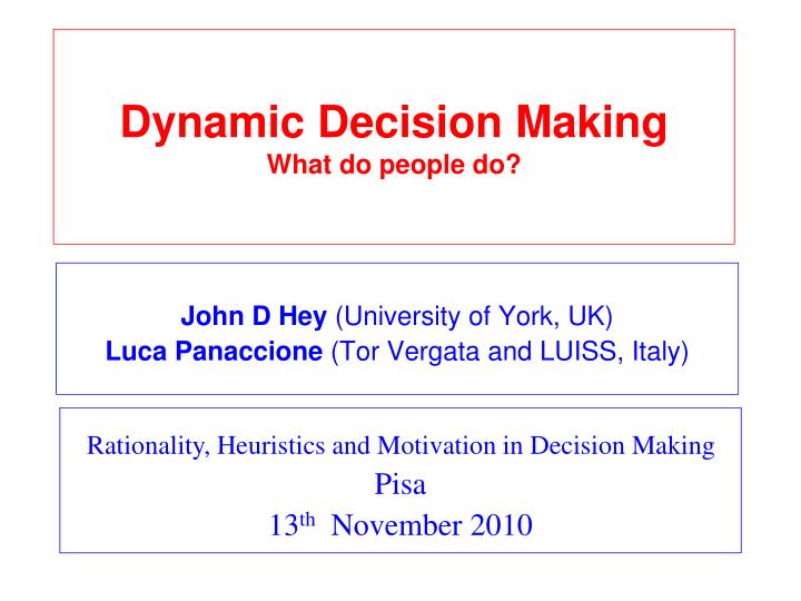
Dynamic Decision Making What do people do?. John D Hey (University of York, UK) Luca Panaccione (Tor Vergata and LUISS, Italy). Rationality, Heuristics and Motivation in Decision Making Pisa 13 th November 2010. Background and Motivation.

E N D
Dynamic Decision MakingWhat do people do? John D Hey (University of York, UK) Luca Panaccione (Tor Vergata and LUISS, Italy) Rationality, Heuristics and Motivation in Decision Making Pisa 13th November 2010
Background and Motivation • This project tries to see how potentially dynamically inconsistent people take dynamic decisions: do they act sophisticatedly (as economics usually supposes), resolutely, naively or myopically? • It is a follow-up to Hey and Lotito (2009), JRU. • This new paper has a greatly simplified experimental design. • It is relevant both for discounting problems and for dynamic decisions under risk.
As Wikipedia says: "In economics, dynamic inconsistency, or time inconsistency, describes a situation where a decision-maker’s preferences change over time, such that what is preferred at one point in time is inconsistent with what is preferred at another point in time. It is often easiest to think about preferences over time in this context by thinking of decision-makers as being made up of many different "selves", with each self representing the decision-maker at a different point in time. So, for example, there is my today self, my tomorrow self, my next Tuesday self, my year from now self, etc. The inconsistency will occur when somehow the preferences of some of the selves are not aligned with each other."
Structure of presentation • The problem of potentially dynamically inconsistent people. • The old design (Hey and Lotito). • The new design (Hey and Panaccione). • The experiment. • Results. • Conclusions.
Dynamic decision making • Economists perceive of this being done either by the Strategy Method or by Backward Induction. • If the decision-maker is dynamically consistent (discounts exponentially and/or is EU) then the two methods lead to the same decisions. • If not dynamically consistent, they may lead to different decisions.
Two Problems: what would you choose – Up or Down – in each? £30 £30 Consider a person who violates EU, choosing Up in the first problem and Down in the second. Note: greensquares are decision nodes and red squares are chance nodes. 0.25 first 0.75 £0 £50 £50 second 0.8 0.2 0.8 0.2 £0 £0
What does such a person do in this dynamic problem?Suppose that he/she prefers £30 to the 80% chance of £50 and that he/she strictly prefers the 20% chance of £50 to the 25% chance of £30. Note: greensquares are decision nodes and red squares are chance nodes.
What they do depends on their type • Resolute: Choose Up at the first and Up at the second (even though they want to choose Down when they get there). • Naive: Choose Up at the first and Down at the second. • Sophisticated: Choose Down at the first (because they anticipate moving Down at the second if they choose Up at the first). The latter is what is assumed when backward induction is used.
The old design (Hey and Lotito) • Three sets of four trees, all with the same structure as in the following slide. • Subjects were asked to bid for each tree (so we could observe their valuation) and then play out each of the trees (so we could observe their choices). • We then estimated three models for each subject (naive, resolute and sophisticated) to see which best explains their behaviour. • We found very few sophisticates.
The new design (inspired by Loomes 1991) • Subjects were asked to allocate money between Left and Right (twice) in the following problem. • This problem has two stages: first, the subject allocates money to Left and Right; then Nature moves Left or Right (with stated probabilities); then the subject allocates the money that is left to Left and Right and then Nature moves Left or Right (with stated probabilities). The subject gets the money that is implied.
Types • Resolute: Takes a decision at the first node and then implements it. • Naive: Takes a decision at the first node and may change his or her mind at the second. • Sophisticated: Anticipates his or her decision at the second node and takes that into account when choosing at the first node. • Myopic (a new type): Treats the first decision as the final decision. In other words, ignores the second decision when taking the first.
The problems in the experiment • Each problem is characterised by an amount to allocate (always €40), and three probabilities. • The idea is to choose problems that enable good discrimination between the various types. • As in Hey and Lotito, we have to assume a particular preference function. • We chose RDEU with CRRA utility function (parameter r) and Quiggin weighting function (parameter g). • We then carried out extensive simulations. • (Note that we will explain our parameter notation later. Briefly r is the parameter of the utility function, g the parameter of the weighting function and s the precision.)
Average maximised log-likelihoodsTrue values: r = 2.0, g = 0.8 and s = 75
Standard deviation of maximised log-likelihoodsTrue values: r = 2.0, g = 0.8 and s = 75
Percentage of incorrect types identifiedTrue values: r = 2.0, g = 0.8 and s = 75
The actual implementation • 27 problems • We forced subjects to wait 45 seconds before confirming their decisions on the first stage.. • ..and 15 on the second. • We had 71 subjects, all proceeding at their own pace. • The experiment lasted between 45 minutes and an hour, including reading the instructions. • We paid out just under €20 per subject on average. • (If they were risk-neutral expected payment = €25.)
Example (left allocations) • parameters: r=2.0 g=1.4
Analyses of the data • We fitted RDEU models to the choices of each subject individually (because they are clearly different) assuming each of the four types… • …and we saw which type fitted best. • We assumed a CRRA utility function and a “Quiggin” weighting function. • Details on the next slide…
Utility and weighting functions • CRRA utility function: • u(m) = (m1-1/r-1)/(1-1/r) for r ≠ 1 ln(m) for r = 1 • “Quiggin” weighting function: • w(p) = pg/[(pg+ (1-p)g]1/g • (Note that, if g =1, then RDEU reduces to EU.)
Optimal strategies (for RDEU depend on the ranking of the outcomes) • EU: • RDEU: • Resolute: • Naive: as above then similar to EU • Sophisticated: • Myopic: EU adapted for just one stage.
Stochastic specification 1 • To proceed to the maximum likelihood estimation, we need to assume some stochastic specification. • All the decisions are to do with the proportions of money allocated. • We assume that the actual proportions are all Beta distributions with parameters αand β.
Stochastic specification 2 • The mean of such a distribution is α/(α+β) and the variance is αβ/[(α+β)(α+β+1)]. • If we want these to equal R*and R*(1-R*)/s for some R*and s, we need to put α = R*(s-1) and β = (1-R*)(s-1). • Let R* be the optimal proportion and R the actual proportion, then we assume that each R has a beta distribution with the above parameters. We estimate α, βand s.
Stochastic specification 3 • Notice the nice properties of this… • … there is assumed to be no bias in their allocations… • … and if the optimal proportion is either 0 or 1 (that it, it is optimal to allocate nothing or all) then subjects do not make any errors when implementing this decision. • s is an indicator of the precision.
Stochastic specification 4 • There is one final consideration… • … in the experiment subjects were restricted to integer amounts allocated to the various options… • … while the above stochastic specification is continuous. • We therefore used a discretised version, with the likelihood expressed in probabilities rather than probability densities.
Overview • So for each subject and for each type we have: • estimated values of r, g and s, • the standard errors of the estimates, • and the maximised log-likelihood… • … through which we can compare the goodness of fit of the various types… • … and hence identify which type is ‘best’.
Tests • In order to decide whether one maximised log-likelihood is significantly higher than another, we employed Clarke tests (rather than Vuong tests), based on the statistic: • Clarke shows that:
Conclusions • The bottom line is that the majority of our dynamically inconsistent subjects are resolute, a significant minority are sophisticated; and rather few are naive or myopic. • Software encouraged this? We think not. • Extensions: (1) more and more representative subjects; (2) more stages.