Download
1 / 22
220 likes | 334 Vues
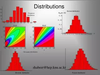
DISTRIBUTIONS. class of “Experimental Methods of Physics” Mikhail Yurov Kyungpook National University April 18 th , 2005. Contents. Introduction Binomial distribution Poisson distribution Gaussian or Normal distribution Gaussian distribution in two variables

E N D
DISTRIBUTIONS class of “Experimental Methods of Physics” Mikhail Yurov Kyungpook National University April 18th, 2005
Contents • Introduction • Binomial distribution • Poisson distribution • Gaussian or Normal distribution • Gaussian distribution in two variables • The relationship among the basic distributions
Introduction Statisticsdeals with random processes. The outcomes of such processes fluctuate from trial to trial, and it is impossible to predict with certainty what the result will be for any given trial. Random processes are described by a probability density function P(x). It gives the expected frequency of occurrence for each possible outcome. The outcome of a random process is represented by a random variable x, which ranges over all possible values in the process. The random variable x is the said to be distributed as P(x). Example: x may take on the integer values from 1 to 6, the probability of an outcome x is given by density function P(x)=1/6, the same for all x in this case
Depending on the process, a random variable may be continuousor discrete. If x is discrete, P(xi) then gives the frequency at each point xi. If x is continuous, this interpretation is not possible and only probability of finding x in finite intervals (x and x+dx) have meaning. The distribution P(x) is then continuous density such that the probability is P(x)dx. Very often it is desired to know the probability of finding x between certain limits P(x1≤x≤x2). This is given by the cumulative or integral distribution. P(x) is continuous P(x) is discrete By convention the probability distribution is normalized to 1 P(x) is discrete P(x) is continuous
Binomial Distribution The binomial distribution applies to situations where we conduct a fixed number N of independent trials. There are only two possible outcomes – success (with probability p) or failure (with probability 1-p). The probability of obtaining r successes is given by For binomial distribution, the expectation value of the number of successes r is The variance of the distribution is given by
The graphs show the probability P of obtaining r success. N is kept fixed at 10, and the two distributions correspond to p=1/2 and 1/4 respectively. The binomial distribution itself is not great application to nuclear physics, since we rarely work with a fixed number of events.
Poisson Distribution The Poisson distribution occurs as the limiting form of the binomial distribution when N→∞ p→0 Such as Np=constant=μt=λremains finite. Then This is the probability of observing r independent events in a time interval t, when the counting rate is μ and the expected number of events in the time interval is λ.
The Poisson distribution is discrete. It essentially describe processes for which the single trial probability of success is very small but in which the number of trials is so large that there is nevertheless a reasonable rate of event. Two important examples of such processes are radioactive decay and particle reaction.
Example Consider a typical radioactive source such as 137Cs which has a half-life of 27 years. The probability per unit time for a single nucleus to decay is then λ=ln2/27=0.026/year=8.2×10-10s-1 However, ever a 1 μg sample of 137Cs will contain about 1015 nuclei. Since each nucleus constitutes a trial, the mean number of decays from the sample will be μ=Np=8.2×10⁵ decays/s This satisfies the limiting conditions describing above, so that the probability of observing r decays is given by formula for Poisson distribution.
It is important to remember that if the rate of the basic process changes (as a function of time or of position), then the observed distribution of events may not follow the Poisson distribution. Example The number of people who die while operating computers each year is not Poisson distribution since although the probability of dying may remain constant, the number of people who operate computers increases from year to year. An important feature of the Poisson distribution is that it depends on only one parameter: μ We also can find that σ2=μ that is the variance of the Poisson distribution is equal to the mean. The standard deviation is then
Gaussian or Normal Distribution The Gaussian or normal distribution plays a central role in all of statistics and is the most ubiquitous distribution in all the sciences. Measurement errors and instrumental errors are generally described by this probability distribution. The Gaussian is a continuous, symmetric distribution whose density is given by The two parameters μ and σ2can be shown to correspond to the mean and variance of the distribution.
The Gaussian distribution for various σ. The significance of σ as a measure of the distribution width is clearly seen. The standard deviation corresponds to the half width of the peak at about 60% of the full height. In some applications, however, the full width at half maximum (FWHM) is often used instead.
This is somewhat larger than σand can be shown to be In such cases, care should be taken to be clear about which parameter is being used.
The integral distribution for the Gaussian density cannot be calculated analytically so that one must resort to numerical integration. Tables of integral values are readily found as well. These are tabulated in terms of a reduced Gaussian distribution with μ=0 σ2=1 All Gaussian distributions may be transformed to this reduced form by making the variable transformation where μ and σ the mean and standard deviation of the original distribution. It is possible to verify that z is distributed as a reduced Gaussian.
An important practical note is the area under the Gaussian between integral intervals of σ. The presentation of a result as x±σ signifies that the true has ≈68% probability of lying between the limits x-σ and x+σ or a 95% probability of lying between x-2σ and x+2σ, etc. For a 1σ interval, there is almost a 1/3 probability that the true value is outside these limits. If two standard deviations are taken, then, the probability of being outside is only ≈5%, etc.
Gaussian Distribution in two variables For two variables, we have probability distributions given by and Now if x and y are independent we can obtain
This will be down on the probability at the origin by a factor √e when This is to be compared with the corresponding fact that in the 1-dimensial case, the probability is reduced by this factor when x=±σ. We can rewrite in matrix notation as Finally we can invert the 2×2 matrix in the above equation to obtain the matrix which is known as the error matrix for x and y.
The relationship among the basic distributions N→∞, Np=μ Binomial Poisson N→∞ μ→∞ Gaussian
Binomial distributions, characterized by the number of trials N and the probability of success p. Here p is kept constant. The probability P is plotted on a logarithmic scale. As N becomes large, the distributions tend to the inverted parabola shape of a Gaussian distribution of mean Np and variance Np(1-p).
Three binomial distributions in which N increases, but p correspondingly decreases such that Np is constant (and equal two). For large N, these tend to the Poisson distribution with mean and variance Np. For the N=30 case, the binomial probabilities are barely distinguishable (on the scale shown) from the corresponding Poisson distribution.
Comparison of Poisson and Gaussian distributions when the mean is two (open circles for Poisson, solid curve for Gaussian) and five (crosses and dashed curve). This is the basis of the rule of thumb that five events are sufficient to pretend that errors are Gaussian distributed.
References • L.Lyons, “Statistics for nuclear and particle physics”, Cambridge (1985) • William R.Leo “Techniques for Nuclear and Particle Physics Experiments”, Springer-Verlag Berlin Heidelberg (1987) • http://www.stats.gla.ac.uk/steps/glossary/probability_distributions.html