Download
1 / 48
510 likes | 975 Vues
CHAPTER 6 COST ESTIMATION. Jinashree Rajendrakumar Jisha Nambiar Madhuri Chakraborty Priyanka Tyagi Shalini Singh. CASE 6.2. Case 6.2 – The Pump Division. The Pump Division has one plant dedicated to the design & manufacture of pumps. Typical production cycle of a pump is 1-3 years.

E N D
CHAPTER 6COST ESTIMATION Jinashree Rajendrakumar Jisha Nambiar Madhuri Chakraborty Priyanka Tyagi Shalini Singh
Case 6.2 – The Pump Division • The Pump Division has one plant dedicated to the design & manufacture of pumps. • Typical production cycle of a pump is 1-3 years. • Job is highly technical & customized. • Orders are obtained through bids (based on cost estimate) and negotiation sessions. • The contracts generally are fixed price. • Sometimes orders accepted as loss leaders. • High risk of job cost overruns.
Examples (In thousands) Job 1 Job2 Original Cost Estimate $2,113 $1,800 Costs Incurred to date: Manufacturing 2,100 - Engineering 373 100 Estimate to complete 367 2,500 Total current Estimate 2,840 2,600 Lower-of-cost-or-market: Contract sales price 2,520 2,000 Less 10% Allowance for Normal Profit Margin (252) (200) Inventory Value 2,268 1,800 Inventory Reserve Adjustment (loss) (572) (800)
Current Problems in the Department • Final job costs significantly varied from original cost estimates. • Major decline in profitability, combined with several unfavorable year-end “surprise” inventory adjustments. • As company policy is to record revenue & costs on a completed contract basis, it is difficult to determine early, the variances between job costs & estimates.
Some unanswered Questions ? • It is clear from the table, Job-Order costing is being used as each job is customized. But is job-order costing being used within the departments (Engineering, Manufacturing etc) ? • What allocation base/cost driver is being used for applying overhead costs? • What estimation method (High-Low or Regression Analysis) is being used for overhead costs? • How is Under or Over applied Overhead Balances being disposed (Closed out to Cost of goods sold or Allocated between accounts)?
Inventories • Valuation of the Inventory - FIFO, LIFO or Weighted Average Method • Inventory Adjustments The accounting procedures include two year-end adjustments to be made prior to the close of the fiscal year: • Adjusting inventory to physical count: Perform an annual physical inventory count of inventories and reconcile the changes with the inventory balance. • Adjusting the inventory reserve balance: Departments may be required to maintain an inventory reserve. Reserves must be at least equal to and may not exceed the physical inventory by more than 15%. Therefore, if the reserve account is less than the physical inventory count or is more than 15% greater than the physical inventory you will need to adjust the reserve balance. (NOTE: Departmental storerooms using a periodic inventory system are not required to keep a reserve.)
What courses of action appropriate for plant manager & his controller relating to Estimating Costs • Cost estimation team should include Engineering, Design and Manufacturing representatives. Cost estimation should be cross-disciplinary for better accuracy and insight. • Sales department should be given the threshold cost of the project and be trained to negotiate on more favorable payment terms. • Cost Estimate should be updated to reflect new information, given a project’s phase of planning and/or execution. • Plant Manager should review the cost estimates and actual costs more frequently to track variances. • Controller should record costs as a percent of completion rather than on a completed contract basis.
Contd.. • Since the PLC of the jobs are usually 1-3 yrs, the cost estimates should incorporate future costs such as risk contingency costs for major cost elements. • Cost estimation should build in inflation into the cost estimates using Index. Historical data can be used to load the estimates for inflation. • Perform a risk assessment on the entire project in order to define and quantify the potential risk areas and types. • Cost estimation methods used should be consistent, thorough and traceable.
Lower of Cost or Market value • LCM requires that inventory be reported in the financial statements at whichever is lower – its historical cost or its market value. Also damaged or obsolete inventory is written-off in LCM. • The loss (market value < historical cost) must be charged against revenues of the period. Cost of goods sold will absorb the inventory write-down. • The replacement cost (market value) must lie between a ceiling and a floor amount. • The ceiling is the net realizable value(selling price less disposal cost). • The floor is the net realizable value less a normal profit margin. • If cost is lowest of the four values (cost, replacement cost, ceiling, floor), use cost. Otherwise use the second lowest value.
What courses of action appropriate for plant manager & his controller relating to the application of LCM rule • This method applies to the following: - Goods purchased and on hand - The basic elements of cost (direct materials, direct labor, and an allocable share of indirect costs) of goods being manufactured and finished goods on hand • This method does not apply to the following and must be inventoried at cost: - Goods on hand or being manufactured for delivery at a fixed price on a firm sales contract (that is, not legally subject to cancellation by either you or the buyer) - Goods accounted for under the LIFO method (www.irs.gov) • The Pump Division should have an accurate cost estimation method in place and try to avoid “whatever it takes to get the order” practice.
What is the significance of the following methods on the performance of the operation? • Progress Payments • Advance Payments • Escalation Clauses
Progress Payments • Payment on basis of percentage or stage of completion • Payments are based on costs incurred as work progresses • Progress payments are currently limited to 80 percent of incurred costs • Contractors must have approved accounting systems • Advantageous from a cash flow perspective • Improves the working capital of the firm • Progress payments can decrease interest expense • Important for long term contracts • Information is critical for effective contract administration and for audit and investigative purposes
Advance Payments • Advance payments are prepayments and cash advances for the manufacturer to start the job, buy materials and begin production • Advance payments if partial payments or progress payments are not feasible and private financing is not available • Contractors must have approved accounting systems
Escalation clause Definition: A clause in a contract that allows the seller to be offered a higher price should the buyer or another party make a higher bid in the market within a certain period. Contracts can also be indexed for inflation or cost increases.
Benefits of escalation clause • Effective method of coping with inflation • Hold significance for long term contracts • Price adjustment clauses for long-term contracts • Identifies the item(s) that are subject to the escalation clause • The escalation clause should specify frequency for price adjustment • Price index for the calculation of price adjustments (PPI) • Transfers the burden of the price hike to the buyer • Corrects the distortion in the cost estimations
The Brenham General hospital prepares in-house meals for its patients The hospital is facing steady decline in revenues and wanted to cut costs wherever possible It is approached by a Health Food Inc . Which offers it meals @ $11.50 BG Hospital wants to have some idea about the cost of their in-house meal service Based on that they wanted to decide whether to accept the proposal of HFI or not Case 6-1(Background)
High Low Method • The high-low method is based on the rise-over-run formula for the slope of a straight line. It uses two points to estimate the general cost equation Y = a b H • H= the cost driver • Y = dependent variable Variable Cost (Y) = Change in Cost Change in Activity Fixed Cost (H) = Total Cost – Variable Cost
Simple Regression • A regression analysis has two types of variables: • The dependent variable is the cost to be estimated • The independent variable is the cost driver used to estimate the value of the dependent variable • Evaluating a regression analysis: R2, the coefficient of determination, is a measure of the explanatory power of the regression, the degree that changes in the dependentvariable can be predicted by changes in the independent variable. The t-value is a measure of the reliability of each of the independent variables.
Very simple to apply Least expensive A critical defect – uses only two data points Periods in which activity level is unusually low/high will produce inaccurate results. Most accurate and Most costly Complex and involves numerous calculations but principle is simple. Spreadsheet programs now available to handle the complexities. High –Low Method Simple Regression
Other staff =1.52 Days +1021.36 Food Cost =7.00Days Maintenance =0.36 Days +903.48 Equipment = 0.86Days + 460.48 Dietitian = 2875 Total cost= 9.74Days+5250.32 Other Staff = 1.35 Days +1051.7 Food Cost = 6.94 Days + 69.75 Maintenance = 0.32 Days + 915 Equipment = 0.722Days + 490.31 Dietitian = 2875 Total cost = 9.35Days +5401.76 High –Low Method Simple Regression Regression analysis is a better cost estimation method
Other Staff X Food Cost X Maintenance X Equipment X Dietitian X $11.50Per meal X=Services utilized by the respective proposals X X X X In house food serviceHealth Food Inc
Other Staff V+F Food Cost V+F Maintenance V+F Equipment V+F Dietitian F $11.50 /Meal V=Variable & F=Fixed Cost F F F V In house service Health food Inc. Figures in italics and underlined are not considered for comparison because they are common between the options
Compare the two options • Cost of In-house meals Equation=1.35Days+1051.7+6.94Days+69.75+0.32Days+0.722Days Cost = 9.33 Days +1121.45 • Cost of HFI ‘s Proposal Cost = $11.50 per meal
Comparing variable component of two options • In-house meal costs = $9.33 per patient day • HFI’s proposal = $11.50 per meal (1 patient day =2.8 meals ) • HFI’s proposal = $11.50 *2.8 = $32.20 per patient day Conclusion: In-house meal preparation is cheaper
Comparison of total cost of the options using two different occupancy levels
APPLYING OVERHEAD: HOW TO FIND THE RIGHT BASES AND RATES?Overview Application of “Regression Analysis” to determine the relationship between the overhead costs and the cost drivers/ application bases Selection of application bases that reflect the causes of overhead costs Using data and an objective tool to understand the relationships Using the regression results of rates to ABC models. Using regression analysis for construction of multiple overhead rate
What is Regression analysis used to accomplish in this article? PURPOSE: Determine the relationship between the overhead costs and the various cost drivers using regression analysis Identify the application bases/cost drivers that better reflect the causes of the overhead costs Select proper bases that have strong cause-and-effect relationship with the factory overhead costs using objective technique From a wide selection of application bases three cost drivers were picked for overhead costs in the article direct labor hours machine hours number of production setups
What is Regression analysis used to accomplish in this article? Step 1: searching for a proper base Simple regressions on collected data Three different simple regression analyses were performed R squared values ( explain the variability of FOH costs that can be explained by the independent variable) are as under: R squared or coefficient of determination measures the extent of the relationship between the two variables
What is Regression analysis used to accomplish in this article? Step 2: construction of a single overhead rate Constant refers to the estimate of fixed portion of FOH costs X coefficient is an estimate of the variable FOH costs The regression equation: Monthly overhead costs (OH) = $72,794+ $74.72 (MH) fixedvariable
What is Regression analysis used to accomplish in this article? Step 2: contd.. Assign the fixed portion of the overhead costs to the products and jobs using a separate base Find a separate base that reflects the demands made by the products and jobs on the fixed resources. Use two rates for applying OH costs based on two different bases - one for fixed component - one for variable component
What is Regression analysis used to accomplish in this article? Step 3: Construction of multiple overhead rate Variable overhead costs may be driven by several equally important factors Using more than one base for application of overhead costs will give more accurate cost estimates. Perform a multiple regression to construct more than one overhead rate - Machine hours (0.77) Number of setups (0.39) Use FOH costs observations as “Y-Range” and select the range of observations for both machine hours and no. of setups for “X-Range”
What is Regression analysis used to accomplish in this article? Step 3: Construction of multiple overhead rate Regression Equation: OH = $19,796.43+ $65.44 MH + $322.21 NS - monthly total fixed OH costs = $19,796.43 variable OH costs = $65.44 per Machine hour + $322.21 per setup R squared of multiple regression using MH and NS > R-squared of simple regression for MH. ( 0.95 vs 0.77) Variable OH costs based on both machine hours and no of setups would give more accurate estimates Total fixed costs may be applied using a separate base.
What is Regression analysis used to accomplish in this article? Step 3: Construction of multiple overhead rate Reliability of the multiple regression No of observations used 12 t value = X coefficients/ Std error of the Coef t critical = 2 ( general rule 2 indicates highly reliable estimate) t value for machine hours = 9.7 (65.44/6.74) t value for no of setups = 5.49 (322.21/58.66)
What is Regression analysis used to accomplish in this article? Step 4: Rates for activity based costing Regression analysis is used to investigate the strength of the relationship between the various activities and cost drivers for selection of proper bases. To classify a large no of activities into a few groups (cost pools) based on common bases/drivers Use simple regression to study the relationship between activities and cost drivers. Based on R squared values, group activities into cost pools which have common bases/cost drivers. Regression analysis is practical, effective and objective simple when powered by Excel!!!
What are the steps to perform a simple regression analysis? Collect actual data on selected variables for several periods. Ensure consistency in period: daily, weekly, monthly Tabulate dependent (Y) and independent (X) variable on a spreadsheet. Use the Tools–data analysis-regression The window will ask to specify X and Y variable to perform regression. Interpret the regression results Use regression equation to estimate
What does Table 4 tell you? … there is no table 7 • Table 4 gives the relationship between the cost type/activities and the cost drivers. • It gives the strength of the relationship between the cost driver and the activities. Explains how much of the variability of the cost type can be explained by the cost driver.
Which cost driver would you pick for each cost type? • The cost drivers having higher R squared values indicate “stronger” causal relationship. • According to this analysis, the cost driver would be: • Machine hours – Maintenance and Production Scheduling • Pounds of materials – Packaging, Materials handling, Storage