Download
1 / 64
660 likes | 864 Vues
Rietveld texture analysis of SKAT diffractometer data. R.N. Vasin. STI-2011, 6-9 June, 2011, Dubna, Russia. SKAT texture diffractometer. Beamline 7a of IBR-2 . Main objectives : investigation of crystallographic textures of rocks and engineering materials. Total flight path: 103.8 1 m .

E N D
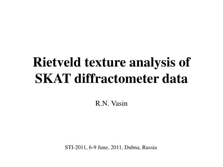
Rietveld texture analysis of SKAT diffractometer data R.N. Vasin STI-2011, 6-9 June, 2011, Dubna, Russia
SKAT texture diffractometer Beamline 7a of IBR-2. Main objectives: investigation of crystallographic textures of rocks and engineering materials. Total flight path: 103.81m. Range of d-spacings: 0.6-4.8 Å. Resolution Δd/d up to 0.55% (d ≈ 2.2 Ǻ). 19 3He detectors on the mounting ring, unique scattering angle of 2θ= 90.
Geometry of diffraction experiment on the SKAT Acquisition of experimental pole figures A S S A S A Schematic view of the SKAT detector system. Usually, 19 detector modules are used. They are named from A to S, with S in the center of the pole figure. The line on the unit sphere corresponds to scattering vectors of the detector ring, the line in theXYplane is its stereographic projection. The grid of the measured pole figure. Small circle correspondsto the plane projection of the scattering vectors, dots shown where the data on pole density are situated.
Data processing Neutron diffraction spectra: 1368 (19 detectors * 72 sample positions)spectra in case of regular 5х5º PF grid Complete experimental pole figures (measured simultaneously - TOF-method!) in regular 5х5º grid Recalculation of the ODF Recalculation of non-measured pole figures using the ODF (absent reflections, overlapped peaks, out of diffractometer’s d-range) ODF characterization: texture index, entropy, construction of the ODF-histogram and ODF-spectrum Calculation of bulk physical properties, application in residual stress measurements, etc.
Data processing: construction of experimental PF We have: raw SKAT data (1368 datafiles: binary, big-endian, 6200 bytes + SKAT protocol file: plain text, contains monitor counts). Front-end processing. Conversion tolittle-endian (from least- to most-significant byte)order, assortment of files into subdirectories, extraction of monitor counts from the protocol file, summation/normalization of spectra are performed. Quartzite Quartz, P3221 Sum of 1368 spectra Diffraction peaks (+ background intervals in vicinity) are selected forPF construction. What are those peaks? Determination of the phase/mineral (in case of poly-phase material) and Miller indices for chosen diffraction peaks.
Data processing: construction of experimental PF Quartzite Quartz, P3221 Determination of the phase and Miller indices for chosen diffraction peaks: comparison with the database. In general, intensive non-overlapped peaks of the single phase are needed!
Data processing: construction of experimental PF Biotite gneiss: Quartz, P3221,SiO2 Biotite, С2/c, K(Mg,Fe,Ti)3(AlSi3O10)(F,OH)2 Plagioclase, P-1, (Ca,Na)(Al,Si)4O8 Intensive non-overlapped peaks of the single phase?? – maybe at d > 3.5 Å (TOF > 2100)…
Data processing: construction of experimental PF PF visualization, rotation, normalization, ... Construction of experimental PF from chosen diffraction peaks (in SKAT grid) Conversion (interpolation) of experimental pole figures into regular 5х5° grid. Conversion of datafiles with PF corresponding to onephaseinto some conventional format:structural info is needed (Laue class, cell parameters, ratio of structure factors for overlapped peaks ofthis phase). For example: shortBerkeley program for conversion into standard Berkeley-format (serves as input in BEARTEX). Repeat for each phase.
Orientation distribution function calculationfrom experimental PF + some other options BEARTEX (WIMV method) H.-R. Wenk & S. Matthies http://eps.berkeley.edu/~wenk/TexturePage/beartex.htm Operations with ODF, PF, inverse PF, PF modeling, tensor averaging (calculation of physical properties), … Single license – 2000$ (academic – 1000$) Someroutinesdo not functionin64-bitOS! LABOTEX (ADC method) K. Pawlik http://www.labosoft.com.pl/index.htm Operations with ODF, PF, inverse PF, … Single license – 6000$ (academic – 3000$)
Standard data processing procedure Raw SKAT data Front-end processing Selection of diffraction peaks for use in the construction of experimental PF Comparison with the database (containing model spectra) Are these peaks present in database? Search for the structural info, load it into database No ODF of each phase Yes Is there enough non-overlapped diffraction peaks for each phase? No No Is there a good agreement between experimental and recalculated PF? Yes Yes Construction of experimental PF, PF conversion into conventional format, ODF reconstruction
Standard data processing procedure: drawbacks • Evident problems with the selection of non-overlapped intensive peaks from diffraction patterns in case of multiphase sample (especially if several low-symmetry phases are present). Usually in this casediffraction peaks are selected at high-d region, where counting statistics are not so good. • Only a small part of acquired diffraction patterns is used (≤6 peaks for each phase). And, for example,for Ni (space group Fm-3m) in SKATd-range at least 12peaks are easily available, for oligoclase An16 (space group P-1) in interval d> 1.5 Å – more than 400 peaks. • The result of the standard data processing is the ODF, no additional information is retrieved (like cell parameters, phase volume fractions, etc.) • New detector rings for SKAT (at different scattering angles) may add some complexities. Solution: it is possible to use Rietveld method for simultaneous processing of all (e.g., 1368) SKAT spectra with account for crystallographic texture (this is requirement!). No need for manual peak selection, most part of available data is used, additional info about crystal structure of the sample is received.
MAUD http://www.ing.unitn.it/~maud/ L. Lutterotti, "Total pattern fitting for the combined size-strain-stress-texture determination in thin film diffraction“, Nuclear Inst. and Methods in Physics Research, B, 268, 334-340, 2010. Freeware! Java-based, needs JVM to work, but this exists for very much every system. Versions for Windows, Mac OS, Linux, Unix (x86 и x64) are available. User-friendly (fine GUI). It’s possible to work with X-ray /synchrotron, electron, neutron diffraction patterns (TOF is included). Great options for texture evaluation: ODF calculation from the set of diffraction spectra (several methods are available).
MAUD And what about TOF spectra?
SKAT data analysis by MAUD: what do we need? • SKAT instrument parameter file (TOF channel tod conversion: scattering angle, delay, DIFC constant ~ L·sinθ; effective spectrum; peak shape)in GSAS format (.prm). • Calibrations have been made for each of 19 detectors of the SKAT (different calibrations for different reactor cycles!); vanadium spectrum have been fitted by FitSpec routine of GSAS, function №4 has been used (MAUD uses functions № 0…5): Maxvellian term + first 10Chebyshev polynomials of the first kind; peak shapehave been approximated by function №1 TOF (the only one available in MAUD???):Gaussian convoluted with two exponentials, accounts only for the instrument-dependent peak broadening in MAUD. • SKAT datafiles in standardGSAS format (.gda) • It’s not a problem to convert binary file to the formatted ASCII with the proper header. But it’s too complicated and time consuming to perform manually for each of 1368 spectra. • Load all the datafiles intoMAUDtaking into account the position on the pole figure (two angles!) and monitor counts. • It’s too complicated and time consuming to perform manually for each of 1368 spectra. The fit is not perfect due to some peculiarities of the vanadium spectrum, its better to use “point-to-point” normalization.
SKAT2MAUD «Mass transformation» of spectra and construction of the specialscript file to automatically load all the data into MAUD. C++ based. Ease to use GUI. Tested inWinXP Pro x86 & Win7 HP x64. File access is made throughWin API functions → it is fast. Conversion + normalization + script creation for 1368 files takes ≈ 15 sec. A possibility to easily add some other IBR-2 diffractometers.
SKAT2MAUD Selection of parameters for the data conversion Spectra selection Monitor counts extraction from the SKAT protocol file Construction of the script file for MAUD and of the protocol. Options for point-to-point data normalization Data type selection
Ni powder The refinement of diffractometer parameters and peak shapes (to get unique parameters for each detector!) Different (most of the time slightly different) parameters for different reactor cycles! Sum spectrum(detectors from A to S)
Ni powder Detector E Detector D Detector C Detector B Detector А
Ni powder (111) peak S (222) & (311) peaks A Detectors:
Neutron diffraction texture analysis of the Outokumpu biotite gneiss 676 Sample: Outokumpu borehole (Finland), 676 m depth. Mineral composition: quartz – 42.6 vol.%, plagioclase – 37.6 vol.%, biotite – 19.8 vol.% (thin sections analysis, Kern, Mengel, Strauss et al. // PEPI, 175, 2009. 151-166). Volume of the sample is > 100 cm3. Lattice spacing range: d = 1.51…4.31 Å → about 700 diffraction peaks/pole figures. Getting prepared for intensive calculations: MAUD command file is altered – now MAUD exclusively allocates 3 Gb ofRAM (should be working on x64 OS orx86 with enabled PAE). Free parameters: phase volume fractions, individual background for each spectrum (3·1386 parameters), cell parameters of each phase, 1 thermal factor for all atoms (isotropic approximation), crystallite size and microdeformation for each phase (isotropic approximation) – in total 4145 parameters. +ODF calculation for each phase, E-WIMV method, 5° ODF resolution, peaks with intensity less than 1% of maximum for the given phase were not used for the ODF calculation. 1 iteration took ≈ 3 h. 40 min. (Intel Core i5-430M, 4 Gb DDR3-1066(CL7), Win7 HP x64, x64 Java Virtual Machine).
Neutron diffraction texture analysis of the Outokumpu biotite gneiss 676 First 12 spectra, detector A, point-to-point normalized in SKAT2MAUD.
Neutron diffraction texture analysis of the Outokumpu biotite gneiss 676 Q(100) + Pl(030) Pl(-201) Q(101) + Q(011) + Bi(600) + Bi(402) + Pl(-112) + Pl(-221) Bi(-411) + Pl(-210) Pl(002) + Pl(-220) + Pl(-1-22) + Pl(040) + Pl(-202)
Neutron diffraction texture analysis of the Outokumpu biotite gneiss 676 SKAT pole figure coverage for the 676 gneiss sample (different colors correspond to different number of counts of the beam monitor).
Neutron diffraction texture analysis of the Outokumpu biotite gneiss 676 Biotite rec. PF, log scale, MAUD (ODF: texture index F2=5.67) 2M1 polymorph (space group C2/c). Setting 1 is used for the monoclinic biotite here and further. Biotite rec. PF, log scale, conventional PF analysis (ODF: texture index F2=3.30)
Neutron diffraction texture analysis of the Outokumpu biotite gneiss 676 Plagioclase rec. PF, MAUD (ODF: texture index F2=1.27) Plagioclase rec. PF, conventional PF analysis (ODF: texture indexF2=1.23)
Neutron diffraction texture analysis of the Outokumpu biotite gneiss 676 Quartz rec. PF, MAUD (ODF: texture index F2=1.24) Quartz rec. PF, conventional PF analysis (ODF: texture index F2=1.30) Are indistinguishable in conventional PF analysis because overlapped PF of rombs – (h0l) + (0hl) – have not been selected for ODF calculation.
Neutron diffraction texture analysis of the Outokumpu biotite gneiss 676 Is it possible to use less data and get the ODF with acceptable resolution? PF coverage (1/20 from the available data). ODF resolution of 7.5° has been chosen in E-WIMV (instead of 5° as it was in the case of full dataset) to account for the decrease in the quantity of data.
Neutron diffraction texture analysis of the Outokumpu biotite gneiss 676 Biotite rec. PF, log scale, full coverage (ODF: texture index F2=5.67) Biotite rec. PF, log scale, reduced coverage, ODF resolution 7.5° (ODF: texture index F2=8.99)
Neutron diffraction texture analysis of the Outokumpu biotite gneiss 676 Plagioclase rec. PF, full coverage (ODF: texture index F2=1.27) Plagioclase rec. PF, reduced coverage, ODF resolution 7.5° (ODF: texture indexF2=1.39)
Neutron diffraction texture analysis of the Outokumpu biotite gneiss 676 Quartz rec. PF, full coverage (ODF: texture index F2=1.24) Quartz rec. PF, reduced coverage, ODF resolution 7.5° (ODF: texture index F2=1.37)
Outokumpu 676 (a comparison of cell parameters with the American Mineralogist crystal structure database)
Neutron diffraction texture analysis of the Outokumpu biotite gneiss818 Sample: Outokumpu borehole (Finland), 818 m depth. Mineral composition: quartz – 39.9vol.%, plagioclase – 37.4vol.%, biotite – 22.6vol.% (thin sections analysis). Volume of the sample is ≈ 100 cm3. Outokumpu 676 Two biotite peaks almost disappear from the sum diffraction pattern of the 818 sample. The reason for this is higher crystal symmetry of biotite in 818 sample: in 676 → C2/c in 818 → C2/m Outokumpu 818
Neutron diffraction texture analysis of the Outokumpu biotite gneiss818 SKAT pole figure coverage for the 818 gneiss sample. Full coverage (72 sample positions). Measurement time: 36 hours. ¼ coverage (18 sample positions). Measurement time: 9 hours. ODF resolution of 5° has been used ODF resolution of 7.5° has been used
Neutron diffraction texture analysis of the Outokumpu biotite gneiss818 Biotite rec. PF, log scale, full coverage (ODF: texture index F2=4.69) 1M polymorph (space group C2/m). Setting 1 is used for the monoclinic biotite. Biotite rec. PF, log scale, ¼ coverage (ODF: texture index F2=6.19)
Neutron diffraction texture analysis of the Outokumpu biotite gneiss818 Plagioclase rec. PF, full coverage (ODF: texture index F2=1.23) Plagioclase rec. PF, ¼ coverage (ODF: texture indexF2=1.20)
Neutron diffraction texture analysis of the Outokumpu biotite gneiss818 Quartz rec. PF, full coverage (ODF: texture index F2=1.16) Quartz rec. PF, ¼ coverage (ODF: texture index F2=1.20)
GEOMixSelf elastic properties calculation of the Outokumpubiotite gneiss818 (spherical grains, no pores) Full coverage VP VS splitting ¼ coverage, VP velocities change by about 30 m/s ≈ 0.5%, max VS split increase by ≈ 8%
Neutron diffraction texture analysis of the Outokumpu biotite gneiss818: ODF spectra Biotite Full coverage Biotite ¼ coverage
Neutron diffraction texture analysis of the Outokumpu biotite gneiss818: ODF spectra Biotite Full coverage Biotite ¼ coverage
Neutron diffraction texture analysis of the Outokumpu biotite gneiss818: ODF spectra Plagioclase Full coverage Plagioclase ¼ coverage
Neutron diffraction texture analysis of the Outokumpu biotite gneiss818: ODF spectra Quartz Full coverage Quartz ¼ coverage
Neutron diffraction texture analysis of the Outokumpu biotite gneiss818 Full coverage ¼ coverage Phase analysis via thin sections (Kern, Mengel, Strauss et al. // PEPI, 175, 2009. 151-166) • Only notable changes are in cell parameters and texture index of the biotite. This may be due to: • Biotite peaks are the least intensive and they are “lost” in the noisy pattern. • Should account for 1M and 2M1 polymorphs coexistence in the sample?
Outokumpu 818: comparison with the HIPPO data HIPPO PF coverage (includes different detectors on different scattering angles) – by courtesy of Prof. H.-R. Wenk. HIPPO diffractometer (Los-Alamos) Volume of the sample is about 1 cm3! 4 sample positions have been measured, 2 hours per position, in total 8 hours of measurements.
Outokumpu 818: comparison with the HIPPO data Spectra from 90° detectors of SKAT Spectra from 144° detectors of HIPPO
Outokumpu 818: comparison with the HIPPO data Biotite rec. PF, log scale, full coverage (ODF: texture index F2=4.69) Biotite rec. PF, log scale, HIPPO, 10° resolution (ODF: texture index F2=8.90)
Outokumpu 818: comparison with the HIPPO data Quartz rec. PF, full coverage (ODF: texture index F2=1.16) Quartz rec. PF, HIPPO, 10° resolution (ODF: texture index F2=1.18)
Outokumpu 818: comparison with the HIPPO data Plagioclase rec. PF, full coverage (ODF: texture index F2=1.16) Plagioclase rec. PF, HIPPO, 10° resolution (ODF: texture index F2=1.22)
Neutron diffraction texture analysis of the quartzite sample 26а PF coverage used. Only 114 spectra (1/12of the full coverage), sample positions 00 = 0°, 12 = 60°, 24 = 120°, 36 = 180°, 48 = 240°, 60 = 360°. Range of lattice spacingsd = 0.6-3.4 Å (≈ 310 diffraction peaks, i.e., 310 pole figures). ODF was recalculated by the E-WIMV method, 5° resolution, exp. pole figures (100), (110), (012+102). Complete PF measurements took 15 h. 36 min. 1/12 of full coverage was possible to measure in 1 h. 18 min.
Neutron diffraction texture analysis of the quartzite sample 26а Single spectrum, detector A, sample position 12. (012+102) (100) (110)
Neutron diffraction texture analysis of the quartzite sample 26а Quartz rec. PF, MAUD, 1/12 coverage (ODF: texture index F2=2.24) Quartz rec. PF, conventional PF analysis, exp. pole figures (100), (110), (012+102) & WIMV method via BEARTEX (ODF: texture indexF2=2.35)