Download
1 / 28
280 likes | 367 Vues
Artificial emissions and formation of ionized layers in the ionosphere due to HF-heating. G. Milikh (1) , D. Papadopoulos (1) , B . Eliasson (1 ) , Xi Shao (1), and E. Mishin (2) University of MD, College Park (2) Space Vehicles Directorate, Air Force Research Laboratory.

E N D
Artificial emissions and formation of ionized layers in the ionosphere due to HF-heating G. Milikh(1), D. Papadopoulos(1), B. Eliasson(1), Xi Shao(1), and E. Mishin(2) University of MD, College Park (2) Space Vehicles Directorate, Air Force Research Laboratory
Motivations and Objectives Models of electron acceleration due to HF-heating were introduced since 1970-es. However recent optical and ionosonde observations emphasized a need of a comprehensive model of electron acceleration by the Langmuir turbulence due to the ionospheric HF-heating. The objective of this project is to develop such a model and check it against the existing observations.
Model Approach • Describe topside electrostatic turbulence due to HF-heating • Obtain energy spectrum of the electrons accelerated by such turbulence: • - Solving the F-P equation • - Using PIC method • Consider effects on the energy spectrum due to energy losses by the electrons propagating in the ionosphere • Study effects caused by the fast electrons: • - Optical emissions • - Formation of ionized layers
Simulation of topside ionospheric turbulence [Eliasson, 2008, 2010] • A full scale model of the ionosphere is applied, in which O-mode EM wave, is injected from the bottom side. 1D ionospheric density profile has a Gaussian shape, B-field is tilted 14 deg. to vertical. • The mathematical model includes equations for all three E-field components coupled with electron and ion continuity and momentum 1D equations.
Most notably is the strong Ez field at ~230 km which is associated with electrostatic Langmuir waves that have collapsed into solitary wave packets.
Amplitude of Ez-field at different heights, for injected E0=1.5 V/m, O-mode.
Ez at the vicinity of O-mode cutoff, Injected are the waves of 1.0 V/m, 1.5 V/m and 2.0 V/m.
Electron acceleration by quasi-linear diffusion by plasma waves Slowly varying electron distribution function is governed by F-P equation s the spectral density of the electric field per wave number
The energy distribution and integrated density.
Comparing Diffusion Calculation with Particle Tracing Particle Tracing Particle Tracing Diffusion Diffusion f(E) f(E) Initial Thermal E0 = 0.4 eV Initial Thermal E0 = 0.6 eV E (eV) E (eV) Particle Tracing Diffusion f(E) Initial Thermal E0 = 1.0 eV
Modeling Flux Transport Gurevich et al. [1985] showed that propagation of fast electrons outside of accelerating layer is described by the kinetic equation:
E = 1.5 V/m, Simulation for HAARP, E0 = 0.6 eV, Z0= 230 km, O Mode: f(E) for z= 150-230km
E = 1.5 V/m, Simulation for HAARP, E0 = 0.6 eV, Z0= 230 km, O Mode: f(E) for z= 230-380 km
Modeling Optical Emission: Excitation Rate (E = 1.5 V/m, Simulation for HAARP, E0 = 0.6 eV, Z0= 230 km, O Mode)
Model of the column integrated optical emissions of atomic oxygen
Telescopically-imaged heater-induced airglow Stanford/HAARP Photometer
Descending AA 2GH, 440 MW, MZ • Time-vs-altitude plot of 557.7 nm optical emissions along B with contours showing the altitudes where fp =2.85 MHz (blue),UHR= 2.85 MHz (violet), and 2fce = 2.85 MHz (dashed white). Horizontal blips are stars. Shown in greenis the Ion Acoustic Line intensity. • the artificial plasma near hmin was quenched several times. • (left) Background echoes (the heater off). • (center) Heater on: Two lower layers of echoes near 160 and 200 km virtual height for 210 s. • (right) True height profiles. Mishin & Pedersen , GRL 2011 Pedersen et al., GRL 2010
Modeling the ionization wave • The ionization wave occurs in steps, the descending suprathermal electrons ionize the neutral species till the plasma reaches such density that it reflects the HF wave. The reflected wave generates the Langmuir turbulence, leading to the electron acceleration. • A 1D model of a uniform plasma slabs is applied: • The ionization is caused by descending flux of suprathermal electrons (energy losses included) • E-I recombination, charge exchange and ambipolar diffusion all take place inside a slab
Eo= 0.6 eV, E in= 1.5 V/m Kion*Nm*Ne0 Kion
Electron Density Profile Heating layer moved to z= 216 km 10 second each
Conclusions • A model of artificial optical emissions and formation of the ionized layers is discussed • The model is based of the electron acceleration by the Langmuir turbulence caused by HF-heating • The ionization wave which forms the ionized layers occurs in steps • The model will be checked against the existing observations