Download
1 / 39
390 likes | 541 Vues
Protein complexes and their shared components. - Most cellular processes result from a cascade of events mediated by proteins that act in a cooperative manner. Protein complexes can share components: proteins can be reused and participate to several complexes.

E N D
Protein complexes and their shared components • - Most cellular processes result from a cascade of events mediated by proteins that act in a cooperative manner. • Protein complexes can share components: proteins can be reused and participate to several complexes. • Methods for analyzing high-throughput protein interaction data have mainly used clustering techniques. • They have been applied to assign protein function by inference from the biological context as given by their interactors, and to identify complexes as dense regions of the network (see V9). • The logical organization into shared and specific components, and its representation remains elusive. Gagneur et al. Genome Biology 5, R57 (2004) Bioinformatics III
shared components Shared components = proteins or groups of proteins occurring in different complexes are fairly common: A shared component may be a small part of many complexes, acting as a unit that is constantly reused for ist function. Also, it may be the main part of the complex e.g. in a family of variant complexes that differ from each other by distinct proteins that provide functional specificity. Aim: identify and properly represent the modularity of protein-protein interaction networks by identifying the shared components and the way they are arranged to generate complexes. Gagneur et al. Genome Biology 5, R57 (2004) Georg Casari, Cellzome (Heidelberg) Bioinformatics III
Modules A graph and its modules. Nodes connected by a link are called neighbors. In graph theory, a module is a set of nodes that have the same neighbors outside the module. In addition to the trivial modules{a},{b},...,{g} and {a,b,c,..,g}, this graph contains the modules {a,b,c}, {a,b},{a,c},{b,c} and {e,f}. Gagneur et al. Genome Biology 5, R57 (2004) Bioinformatics III
Quotient • Elements of a module have exactly the same neighbors outside the module • one can substitute all of them for a representative node. In a quotient, all elements of the module are replaced by the representative node, and the edges with the neighbors are replaced by edges to the representative. Quotients can be iterated until the entire graph is merged into a final representative node. Iterated quotients can be captured in a tree, where each node represents a module, which is a subset of ist parent and the set of its descendant leaves. Gagneur et al. Genome Biology 5, R57 (2004) Bioinformatics III
Modular decomposition Modular decomposition of the example graph shown before. Modular decomposition gives a labeled tree that represents iterations of particular quotients, here the successive quotients on the modules {a,b,c} and {e,f}. The modular decomposition is a unique, canonical tree of iterated quotients (formal proof exists Möhring 1985). Gagneur et al. Genome Biology 5, R57 (2004) Bioinformatics III
Modular decomposition The nodes of the modular decomposition are labeled in 3 ways: As series when the direct descendants are all neighbors of each other, as parallel when the direct descendants are all non-neighbors of each other, and by the structure of the module otherwise (prime module case). Series are labeled by an asterisk within a circle, parallel by two parallel lines within a circle, and prime by a P within a circle. The prime is advantageously labeled by its structure. The graph can be retrieved from the tree on the right by recursively expanding the modules using the information in the labels. Therefore, the labeled tree can be seen as an exact alternative representation of the graph. Gagneur et al. Genome Biology 5, R57 (2004) Bioinformatics III
Results from protein complex purifications (PCP), e.g. TAP • Different types of data: • Y2H: detects direct physical interactions between proteins • PCP by tandem affinity purification with mass-spectrometric identification of the protein components identifies multi-protein complexes • Molecular decomposition will have a different meaning due to different semantics of such graphs. Here, focus analysis on PCP content. PCP experiment: select bait protein where TAP-label is attached Co-purify protein with those proteins that co-occur in at least one complex with the bait protein. In future, integrated view combining both types of data would be preferred. Gagneur et al. Genome Biology 5, R57 (2004) Bioinformatics III
Clique and maximal clique A clique is a fully connected sub-graph, that is, a set of nodes that are all neighbors of each other. In this example, the whole graph is a clique and consequently any subset of it is also a clique, for example {a,c,d,e} or {b,e}. A maximal clique is a clique that is not contained in any larger clique. Here only {a,b,c,d,e} is a maximal clique. Assuming complete datasets and ideal results, a permanent complex will appear as a clique. The opposite is not true: not every clique in the network necessarily derives from an existing complex. E.g. 3 connected proteins can be the outcome of a single trimer, 3 heterodimers or combinations thereof. Gagneur et al. Genome Biology 5, R57 (2004) Bioinformatics III
Results from protein complex purifications (PCP), e.g. TAP Interpretation of graph and module labels for systematic PCP experiments. (a) Two neighbors in the network are proteins occurring in a same complex. (b) Several potential sets of complexes can be the origin of the same observed network. Restricting interpretation to the simplest model (top right), the series module reads as a logical AND between its members. (c) A module labeled ´parallel´ corresponds to proteins or modules working as strict alternatives with respect to their common neighbors. (d) The ´prime´ case is a structure where none of the two previous cases occurs. Gagneur et al. Genome Biology 5, R57 (2004) Bioinformatics III
Obtain maximal cliques Modular decomposition provides an instruction set to deliver all maximal cliques of a graph. In particular, when the decomposition has only series and parallels, the maximal cliques are straightforwardly retrieved by traversing the tree recursively from top to bottom. A series module acts as a product: the maximal cliques are all the combinations made up of one maximal clique from each „child“ node. A parallel module acts as a sum: the set of maximal cliques is the union of all maximal cliques from the „child“ nodes. Gagneur et al. Genome Biology 5, R57 (2004) Bioinformatics III
Modular decomposition of graphs • The notion of module naturally arises from different combinatorial structures and has been introduced several times in different fields: • Modules have been called Decompositions have also been called • Autonomous sets - substitution decomposition • Closed sets - ordinal sum • Stable sets - X-join • Clumps • Committees • Externally related sets • Nonsimplifiable subnetworks • Partitive sets • … Muller&Spinrad, J. Ass. Comp Mach 36, 1 (1989) Bioinformatics III
Consider undirected graph G=(V,E) with n =|V| vertices and m=|E| edges. The complement of a graph G is denoted by G. If X is a subset of vertices, then G[X] is the subgraph of G induced by X. Let x be an arbitrary vertex, then N(x) and N(x) stand respectively for the neighborhood of x and its non-neighborhood. A vertex xdistinguishes two vertices u and v if (x,u) E and (x,v) E. A moduleM of a graph G is a set of vertices that is not distinguished by any vertex. Bioinformatics III
A simple linear algorithm for modular decomposition The modules of a graph are a potentially exponentially-sized family However, the sub-family of strong modules, the modules that overlap no other modules, has size O(n). AoverlapsB if A B , A \ B and B \ A The inclusion order of this family defines the previously explained modular tree decomposition, which is enough to store the module family of a graph. The root of this tree is the trivial module V and its n leaves are the trivial modules {x}, xV. Habib, de Montgolfier, Paul (2004) Bioinformatics III
Aim: a simple linear algorithm for modular decomposition Any graph G with at least 3 vertices is either not connected or its complement G is not connected or G and G are both connected. In the last case, the maximal modules define a partition of the vertex-set and are said to be a prime composition. The modular decomposition tree can be recursively built by a top-down approach. At each step, the algorithm recurses on graphs induced by the maximal strong modules. This technique gives an O(n4) complexity. Here, derive a linear-time algorithm that computes a modular factorizing permutation without computing the underlying decomposition tree. This tree may be derived in a second step. Habib, de Montgolfier, Paul (2004) Bioinformatics III
Modular decomposition of protein interaction graphs A graph and its modular tree decomposition. The set {1,2} is a strong module. The module {7,8} is weak: it is overlapped by the module {8,9}. The permutation = (1,2,3,4,5,6,7,8,9) is a modular factorizing permutation. Habib, de Montgolfier, Paul (2004) Bioinformatics III
Module-factorizing orders Let G=(V,E) be a graph and let Obe a partial order on V. For two comparable elements x and y where x <O y we state x precedes y and y follows x. Two subsets A and B cross if a,a‘ A and b,b‘ B such that a <O b and a‘ >O b‘. A linear extension of a partially ordered set (‚poset‘) is a completion of the poset into a total order. Definition 1. A partial order O is a Module-Factorizing Partial Order (MFPO) of V(G) if any pair of non-intersecting strong modules of G do not cross. The modular factorizing permutations are exactly the module-factorizing total orders. Proposition 1. A partial order O is an MFPO if and only if it can be completed into a factorizing permutation. Habib, de Montgolfier, Paul (2004) Bioinformatics III
Module-factorizing orders Definition 2. An ordered partition is a collection {P1, ..., Pk} of pairwise disjoint parts, with and an order O such that for all x Pi and y Pj, x <O y if i < j. Start with trivial partition (a single part equal to the vertex set) and iteratively extend (or refine) it until every part is a singleton. A center vertexc V is distinguished and two refining rules, preserving the MFPO property, are used. They are defined in Lemma 1: Habib, de Montgolfier, Paul (2004) Bioinformatics III
Defining rules • Lemma 1. • Center Rule: For any vertex c, the ordered partition • is module-factorizing. The center rule picks a center and breaks a trivial partition to start the algorithm. Once launched, the process goes on based on the pivot rule, that splits each part Pi(except the part Pi that contains the pivot), according to the neighborhood of the pivot. Habib, de Montgolfier, Paul (2004) Bioinformatics III
Defining rules: pivot rule Lemma 1 continued. 2. Pivot Rule: Let be an ordered partition with center c and p Pi such that Pj, ij, overlaps N(p) . If O is an MFPO, then the following refinements preserve the module-factorizing property: Habib, de Montgolfier, Paul (2004) Bioinformatics III
Preliminary algorithm Partition refinement scheme that outputs a partition of V into the maximal modules not containing c. When this algorithm ends, every part is a module. To obtain a factorizing permutation it has to be recursively relaunched on the non-singleton parts. Habib, de Montgolfier, Paul (2004) Bioinformatics III
Execution example of algorithm The resulting factorizing permutation is (a, s, v, w, u, y, x, z, t). Habib, de Montgolfier, Paul (2004) Bioinformatics III
Ordered chain partition yields linear-time algorithm Definition 3. An ordered chain partition (OCP) is a partial order such that each vertex belongs to one and only one chain, and one chain belongs to one and only one part. The vertices of the same chain are totally ordered, the chains of the same part are uncomparable, and the parts of totally ordered. A trivial chain contains only 1 vertex, and a monochain part contains only one chain. The OCPs generalize the Ordered Partitions since the latter ones contain only trivial chains. Habib, de Montgolfier, Paul (2004) Bioinformatics III
Ordered chain partition yields linear-time algorithm C(x)denotes the chain containing x while P(x) denotes the part of the partition containing x. Each chain C has a representative vertexr(C) C. During the algorithm, the chains will behave as their representative vertices. Chains are possibly merged. Then, the representative of the new chain is one of the former representatives. But chains will never be split. The algorithm still uses the center and pivot rules. The chains are moved by these 2 rules, according to the adjacency between their representative vertex and the center of the pivot. But there is a third rule, the chaining rule (line 9 of algorithm). Habib, de Montgolfier, Paul (2004) Bioinformatics III
Defining rule 3: Chaining rule There is a third rule, the chaining rule Unlike the two first ones, the third rule removes comparisons from the order. It first concatenates a sequence of monochain parts, that occur consecutively in O, into one chain. Then this new chain is inserted into one of the two parts, say P, neighboring the chain. Chaining rule, chaining the black vertices into P. The comparisons between the chain and P are lost. But since the number of chains strictly decreases during the algorithm, the process is guaranteed to end. Habib, de Montgolfier, Paul (2004) Bioinformatics III
Ordered chain partition yields linear-time algorithm Use each vertex a constant number of times as a pivot. Habib, de Montgolfier, Paul (2004) Bioinformatics III
Execution example of algorithm The resulting factorizing permutation is (a, s, v, w, u, y, x, z, t). Habib, de Montgolfier, Paul (2004) Bioinformatics III
Modular decomposition of protein interaction graphs Finally the following invariant is satisfied: Invariant 1. The ordered chain partition O is an MFPO of V(G) and no chain is overlapped by a strong module. Position of a strong module M (black vertices) in O (Invariant 1). To use any vertex O(1) times as a pivot, the algorithm picks only one vertex per part to extend the OCP. A chain C is ´used´ if its representative vertex r(C) has already been used as pivot by some extension rule. Similarly, a part is ´used´ if it contains a used chain. Pivots may be chosen from `unused` parts only ensuring each vertex neighbor-hood is used O(1) times. The non-trivial (multichain) parts are not necessarily modules. The algorithm chooses a new center and recurses (line 12). Habib, de Montgolfier, Paul (2004) Bioinformatics III
Choice of the new center. The center plays an important role (see Lemma 1). Invariant 2 Let M be a strong module and c be the center. Then either c belongs to M, or M consists in consecutive monochain parts, or M is included in a single part P. The new center cnmust fulfil Invariant 2 as the old center c did. If all the strong modules containing c but not cnare included in P(c) then Invariant 2 holds. Habib, de Montgolfier, Paul (2004) Bioinformatics III
Choice of the new center. Let PL (resp. PR) be the rightmost (resp. leftmost) multichain part that precedes (resp. follows) c. As both parts are `used`, their pivots pL and pR are defined. One of them is chosen for the recursive call, and its pivot becomes the new center. Only one pivot among pLand pRdistinguishes the other from the center c. The rule chooses that pivot as new center. This can be implemented by an adjacency test. … and so-forth … see original article Habib, de Montgolfier, Paul (2004) Bioinformatics III
Implementation of an Ordered Chain Partition Habib, de Montgolfier, Paul (2004) Bioinformatics III
Execution example of algorithm • Summary: • simple, linear-time • algorithm now available • for modular decomposition • of graphs. • What is the meaning of • such modules when • applied to real data? The resulting factorizing permutation is (a, s, v, w, u, y, x, z, t). Habib, de Montgolfier, Paul (2004) Bioinformatics III
Interpretation for PCP protein interaction networks In the modular decomposition tree, the leaves are proteins, the root represents the whole network. In between, each node is a module that is a sub-part of ist parent. The label of a node gives the nature of the relationship between ist direct children. Proteins or modules in a parallel module can be be seen as alternatives. If A is neighbor of B and C, which are not neighbors of each other, then A can belong to a complex together with either B or C, but not with both at the same time. B and C define a parallel module and thus are alternative partners in a complex with their common neighbor A. This situation corresponds to a logical „exclusive OR“ between B and C. Gagneur et al. Genome Biology 5, R57 (2004) Bioinformatics III
Interpretation for PCP protein interaction networks Proteins or modules in a series module can be seen as potentially combined in any way. If A is neighbor of B and C, and B and C are also neighbors, the A can belong to a complex together with B or C, or with both at the same time. This corresponds to a logical „OR“ between B and C. A series module can be seen as a unit: a set of proteins (modules) that function together. A ‚prime‘ is a graph where neither of these cases occurs. Gagneur et al. Genome Biology 5, R57 (2004) Bioinformatics III
Back to the real world … Three examples of modular decomposition of protein-protein interaction networks. In each case from top to bottom: schema of complexes, the corresponding protein-protein interaction network as determined from PCP experiments, and its modular decomposition (MOD). (a) Protein phosphatase 2A. Parallel modules group proteins that do not interact but are functionally equivalent. Here these are the catalytic Pph21 and Pph22 (module 2) and the regulatory Cdc55 and Rts1 (module 3). Gagneur et al. Genome Biology 5, R57 (2004) Bioinformatics III
RNA polymerases I, II and III A good layout of the corresponding network gives an intuitive idea of what the constitutive units of the complexes are. Modular decomposition extracts them and makes their logical combinations explicit. Gagneur et al. Genome Biology 5, R57 (2004) Bioinformatics III
Transcriptional regulator complexes Modular decomposition condenses the network to its backbone prime structure (root of the tree) and identifies its constitutive units. Gagneur et al. Genome Biology 5, R57 (2004) Bioinformatics III
NFB variants Modular decomposition of NFκB members relB, c-rel, p50 and p52 delivers the potential NFκB dimers and tetramers. All combinations are possible (series) except those including both relB and c-rel (parallel), and those including both p50 and p52. Gagneur et al. Genome Biology 5, R57 (2004) Bioinformatics III
Modular decomposition of the network of NFκB members and their partners in resting cells. The network is composed of the NFκB members and their interactors. In this step, interactions among the interactors are disregarded. Baits are outlined in green. Modular decomposition organizes the interactors into modules. The root is a prime whose structure is shown in the encircled network. Module 1 and module 2, respectively, group the new interactors into activators and inhibitors of NFκB. Gagneur et al. Genome Biology 5, R57 (2004) Bioinformatics III
Summary Ongoing: need for modular description of molecular biology. What are suitable modules? Spirin&Mirny, Barabasi et al. : identify dense parts of the network Alon and co-workers: identify (small) repeated motifs Here: apply established method of modular graph decomposition to protein interaction networks. Can (and has been) applied to other networks. What is the biological relevance of modules at different levels? Integrate with gene ontology? Gagneur et al. Genome Biology 5, R57 (2004) Bioinformatics III