Download
1 / 62
700 likes | 1.15k Vues
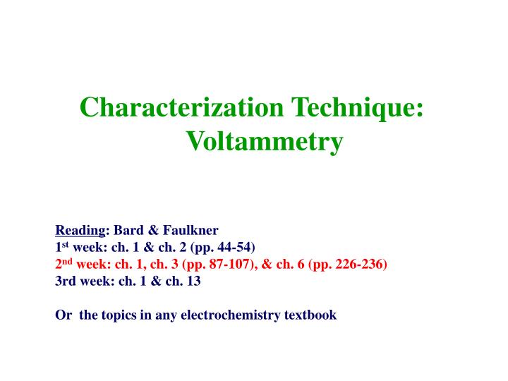
Characterization Technique: Voltammetry. Reading : Bard & Faulkner 1 st week: ch. 1 & ch. 2 (pp. 44-54) 2 nd week: ch. 1, ch. 3 (pp. 87-107), & ch. 6 (pp. 226-236) 3rd week: ch. 1 & ch. 13 Or the topics in any electrochemistry textbook. Current vs. reaction rate i (A) = dQ/dt (C/s)

E N D
Characterization Technique: Voltammetry Reading: Bard & Faulkner 1st week: ch. 1 & ch. 2 (pp. 44-54) 2nd week: ch. 1, ch. 3 (pp. 87-107), & ch. 6 (pp. 226-236) 3rd week: ch. 1 & ch. 13 Or the topics in any electrochemistry textbook
Current vs. reaction rate i (A) = dQ/dt (C/s) Q/nF = N (mol) n: # of electrons in reaction (2 for reduction of Cd2+) Rate (mol/s) = dN/dt = i/nF Electrode process: heterogeneous reaction Rate (mols-1cm-2) = i/nFA = j/nF j: current density (A/cm2) Electrode reaction: i-E curves Polarization: departure of the cell potential from the equilibrium potential Extent of potential measured by the overpotential: = E - Eeq
Factors affecting electrode reaction rate and current 1. Mass transfer 2. Electron transfer at the electrode surface 3. Chemical reactions 4. Other surface reactions: adsorption, desorption, electrodeposition
Review of homogeneous kinetics Dynamic equilibrium kf O + e = R kb Rate of the forward process vf (M/s) = kfCA Rate of the reverse reaction vb = kbCB Rate const, kf, kb: s-1 Net conversion rate of A & B vnet = kfCA – kbCB At equilibrium, vnet = 0 kf/kb = K = CB/CA *kinetic theory predicts a const conc ratio at equilibrium, just as thermodynamics At equilibrium, kinetic equations → thermodynamic ones → dynamic equilibrium (equilibrium: nonzero rates of kf & kb, but equal) Exchange velocity v0 = kf(CA)eq = kb(CB)eq
Arrhenius equation & potential energy surfaces k = Ae–EA/RT EA: activation energy, A: frequency factor Transition state or activated complex → Standard internal E of activation: ΔE‡ Standard enthalpy of activation: ΔH‡ ΔH‡ = ΔE‡ + Δ(PV)‡ ~ ΔE‡ k = Aexp(-ΔH‡/RT) A = A′exp(ΔS‡/RT) ΔS‡: standard entropy of activation k = A′exp[-(ΔH‡ - TΔS‡)/RT] = A′exp(-ΔG‡/RT) ΔG‡: standard free energy of activation
Transition state theory (absolute rate theory, activated complex theory) General theory to predict the values of A and EA Rate constants k = κ(kT/h)e-ΔG‡/RT κ: transmission coefficient, k: Boltzmann const, h: Planck const
Essentials of electrode reactions *accurate kinetic picture of any dynamic process must yield an equation of the thermodynamic form in the limit of equilibrium kf O + ne = R kb Equilibrium is characterized by the Nernst equation E = E0′+ (RT/nF)ln(Co*/CR*) bulk conc Kinetic: dependence of current on potential Overpotential η = a + blogi Tafel equation Forward reaction rate vf = kfCO(0,t) = ic/nFA CO(0,t): surface concentration. Reduction → cathodic current (ic) Backward reaction rate vb = kbCR(0,t) = ia/nFA Net reaction rate vnet = vf – vb = kfCO(0,t) – kbCR(0,t) = i/nFA i = ic – ia = nFA[kfCO(0,t) – kbCR(0,t)]
Butler-Volmer model of electrode kinetics Effects of potential on energy barriers Hg Na+ + e = Na(Hg) Equilibrium → Eeq positive potential than equilibrium negative potential than equilibrium
One-step, one-electron process kf O + e = R kb Potential change from E0′ to E → energy change –FΔE = -F(E – E0′) ΔG‡ change: α term (transfer coefficient) ΔGa‡ = ΔG0a‡ – (1 – α)F(E – E0′) ΔGc‡ = ΔG0c‡ + αF(E – E0′) kf = Afexp(-ΔGc‡/RT) kb = Abexp(-ΔGa‡/RT) kf = Afexp(-ΔG0c‡/RT)exp[-αf(E – E0′)] kb = Abexp(-ΔG0a‡/RT)exp[(1 – α)f(E – E0′)] f = F/RT
At CO* = CR*, E = E0′ kfCO* = kbCR* → kf = kb; standard rate constant, k0 At other potential E kf = k0exp[-αf(E – E0′)] kb = k0exp[(1 – α)f(E – E0′)] Put to i = ic – ia = nFA[kfCO(0,t) – kbCR(0,t)] Butler-Volmer formulation of electrode kinetics i = FAk0[CO(0,t)e-αf(E – E0′) - CR(0,t)e(1 – α)f(E – E0′) k0: large k0 → equilibrium on a short time, small k0 → sluggish (e.g., 1 ~ 10 cm/s) (e.g., 10-9 cm/s) kf or kb can be large, even if small k0, by a sufficient high potential
The transfer coefficient (α) α: a measure of the symmetry of the energy barrier tanθ = αFE/x tanφ = (1 – α)FE/x →α = tanθ/(tanφ + tanθ) Φ = θ & α = ½ → symmetrical In most systems α: 0.3 ~ 0.7
Implications of Butler-Volmer model for 1-step, 1-electron process Equilibrium conditions. The exchange current At equilibrium, net current is zero i = 0 = FAk0[CO(0,t)e-αf(Eeq – E0′) - CR(0,t)e(1 – α)f(Eeq – E0′) → ef(Eeq – E0′) = CO*/CR* (bulk concentration are found at the surface) This is same as Nernst equation!! (Eeq = E0′+ (RT/nF)ln(CO*/CR*)) “Accurate kinetic picture of any dynamic process must yield an equation of the thermodynamic form in the limit of equilibrium” At equilibrium, net current is zero, but faradaic activity! (only ia = ic) → exchange current (i0) i0 = FAk0CO*e-αf(Eeq – E0′) = FAk0CO*(CO*/CR*)-α i0 = FAk0CO*(1 – α) CR*α i0 is proportional to k0, exchange current density j0 = i0/A
Current-overpotential equation Dividing i = FAk0[CO(0,t)e-αf(E – E0′) - CR(0,t)e(1 – α)f(E – E0′)] By i0 = FAk0CO*(1 – α) CR*α → current-overpotential equation i = i0[(CO(0,t)/CO*)e-αfη – (CR(0,t)/CR*)e(1 – α)fη] cathodic term anodic term where η = E - Eeq
Approximate forms of the i-η equation • No mass-transfer effects • If the solution is well stirred, or low current for similar surface conc as bulk • i = i0[e-αfη – e(1 – α)fη] Butler-Volmer equation • *good approximation when i is <10% of il,c or il,a (CO(0,t)/CO* = 1 – i/il,c = 0.9) • For different j0 (α = 0.5): (a) 10-3 A/cm2, (b) 10-6 A/cm2, (c) 10-9 A/cm2 • → the lower i0, the more sluggish kinetics → the larger “activation overpotential” • ((a): very large i0 → engligible activation overpotential)
(a): very large i0 → engligible activation overpotential → any overpotential: “concentration overpotential”(changing surface conc. of O and R) i0 → 10 A/cm2 ~ < pA/cm2 The effect of α
(b) Linear characteristic at small η For small value of x → ex ~ 1+ x i = i0[e-αfη – e(1 – α)fη] = -i0fη Net current is linearly related to overpotential in a narrow potential range near Eeq -η/i has resistance unit: “charge-transfer resistance (Rct)” Rct = RT/Fi0 (c) Tafel behavior at large η i= i0[e-αfη – e(1 – α)fη] For large η (positive or negative), one of term becomes negligible e.g., at large negative η, exp(-αfη) >> exp[(1 - α)fη] i = i0e–αfη η = (RT/αF)lni0 – (RT/αF)lni = a + blogi Tafel equation a = (2.3RT/αF)logi0, b = -(2.3RT/αF)
(d) Tafel plots (i vs. η) → evaluating kinetic parameters (e.g., i0, α) anodic cathodic
Effects of mass transfer Put CO(0,t)/CO* = 1 – i/il,c and CR(0,t)/CR* = 1 – i/il,a to i = i0[(CO(0,t)/CO*)e-αfη – (CR(0,t)/CR*)e(1 – α)fη] i/i0 = (1 – i/il,c)e-αfη – (1 – i/il,a)e(1 – α)fη i-η curves for several ratios of i0/il
Multistep mechanisms Rate-determining electron transfer - In electrode process, rate-determining step (RDS) can be a heterogeneous to electron-transfer reaction → n-electrons process: n distinct electron-transfer steps → RDS is always a one- electron process!! one-step, one-electron process 적용 가능!! O + ne = R → mechanism: O + n′e = O′ (net result of steps preceding RDS) kf O′ + e = R′ (RDS) kb R′ + n˝e = R (net result of steps following RDS) n′ + 1 + n˝ = n Current-potential characteristics i = nFAkrds0[CO′(0,t)e-αf(E – Erds 0′) – CR′(0,t)e(1 – α)f(E –Erds 0′)] krds0, α, Erds0′ apply to the RDS
Multistep processes at equilibrium At equilibrium, overall reaction → Nernst equation Eeq = E0′+ (RT/nF)ln(CO*/CR*) Nernst multistep processes Kinetically facile & nernstian (reversible) for all steps E = E0′+ (RT/nF)ln[CO(0,t)/CR(0,t)] → E is related to surface conc of initial reactant and final product regardless of the details of the mechanism
Mass transport-controlled reactions Modes of mass transfer Electrochemical reaction at electrode/solution interface: molecules in bulk solution must be transported to the electrode surface “mass transfer” Mass transfer-controlled reaction vrxn = vmt = i/nFA Modes for mass transport: (a)Migration: movement of a charged body under the influence of an electric field (a gradient of electric potential) (b) Diffusion: movement of species under the influence of gradient of chemical potential (i.e., a concentration gradient) (c) Convection: stirring or hydrodynamic transport
Nernst-Planck equation (diffusion + migration + convection) Ji(x) = -Di(Ci(x)/x) –(ziF/RT)DiCi((x)/x) + Civ(x) Where Ji(x); the flux of species i (molsec-1cm-2) at distance x from the surface, Di; the diffusion coefficient (cm2/sec), Ci(x)/x; the concentration gradient at distance x, (x)/x; the potential gradient, zi and Ci; the charge and concentration of species i, v(x); the velocity (cm/sec) Steady state mass transfer steady state, (C/t) = 0; the rate of transport of electroactive species is equal to the rate of their reaction on the electrode surface In the absence of migration (excess supporting electrolyte), O + ne- = R The rate of mass transfer, vmt (CO(x)/x)x=0 = DO(COb – COs)/ where x is distance from the electrode surface & : diffusion layer
vmt = mO[COb – COs] where COb is the concentration of O in the bulk solution, COs is the concentration at the electrod surface mO is “mass transfer coefficient (cm/s)” (mO = DO/δ) i = nFAmO[COb – COs] i = -nFAmR[CRb – CRs]
largest rate of mass transfer of O when COs = 0 “limiting current” il,c = nFAmOCOb Maximum rate when limiting current flows COs/COb = 1 – (i/il,c) COs = [1 – (i/il,c)] [ il,c/nFAmO] = (il,c – i)/(nFAmO) COs varies from COb at i = 0 to negligible value at i = il If kinetics of electron transfer are rapid, the concentrations of O and R at the electrode surface are at equilibrium with the electrode potential, as governed by the Nernst equation for the half-reaction E = E0´+ (RT/nF)ln(COs/CRs) E0´: formal potential (activity coeff.), cf. E0 (standard potential) (a) R initially absent When CRb = 0, CRs = i/nFAmR COs = (il,c – i)/(nFAmO)
E = E0´- (RT/nF)ln(mO/mR) + (RT/nF)ln(il,c – i/i) i-E plot When i = il,c/2, E = E1/2 = E0´- (RT/nF)ln(mO/mR) E1/2 is independent of concentration & characteristic of O/R system E = E1/2 + (RT/nF)ln(il,c – i/i)
(b) Both O and R initially present Same method, CRs/CRb = 1 – (i/il,a) il,a = -nFAmRCRb CRs = -[1 – (i/il,a)] [ il,a/nFAmR] = -(il,a – i)/(nFAmR) Put these equations to E = E0´+ (RT/nF)ln(COs/CRs) E = E0´ – (RT/nF)ln(mO/mR) + (RT/nF)ln[(il,c – i)/(i - il,a)] When i = 0, E = Eeq and the system is at equilibrium Deviation from Eeq: concentration overpotential
Potential step experiment Types of techniques Potentiostat: control of potential Basic potential step experiment: O + e → R (unstirred solution, E2: mass-transfer (diffusion)-limited value (rapid kinetics → no O on surface)) chronoamperometry (i vs. t)
-Series of step experiments (between each step: stirring for same initial condition) 4, 5: mass-transfer (diffusion)-limited (no O on electrode surface)) sampled-current voltammetry (i(τ) vs. E) Potential step: E1 → E2 → E1 (reversal technique) double potential step chronoamperometry
Voltammetry Potential Sweep Methods Introduction Most widely used technique Applying a continuously time-varying potential working electrode -oxidation/reduction reactions of electroactive species -adsorption of species -capacitive current due to double layer charging -mechanisms of reactions -identification of species -quantitative analysis of reaction rates -determination of rate constants Two forms: linear sweep voltammetry(LSV) & cyclic voltammetry(CV)
Introduction Linear sweep voltammetry (LSV) Cyclic voltammetry (CV)
Nernstian (reversible) systems Solution of the boundary value problem O + ne = R (semi-infinite linear diffusion, initially O present) E(t) = Ei – vt Sweep rate (or scan rate): v (V/s) Rapid e-transfer rate at the electrode surface CO(0, t)/CR(0, t) = f(t) = exp[nF (Ei - vt - E0′)/RT] i = nFACO*(πDOσ)1/2χ(σt) σ = (nF/RT)v
Peak current and potential Peak current: π1/2χ(σt) = 0.4463 ip = 0.4463(F3/RT)1/2n3/2ADO1/2CO*v1/2 At 25°C, for A in cm2, DO in cm2/s, CO* in mol/cm3, v in V/s → ip in amperes ip = (2.69 x 10⁵)n3/2ADO1/2CO*v1/2 Peak potential, Ep Ep = E1/2 – 1.109(RT/nF) = E1/2 – 28.5/n mV at 25°C Half-peak potential, Ep/2 Ep/2 = E1/2 + 1.09(RT/nF) = E1/2 + 28.0/n mV at 25°C E1/2 is located between Ep and Ep/2 |Ep – Ep/2| = 2.20(RT/nF) = 56.5/n mV at °C For reversible wave, Ep is independent of scan rate, ip is proportional to v1/2
Spherical electrodes and UMEs Spherical electrode (e.g., a hanging mercury drop) i = i(plane) + nFADOCO*φ(σt)/r0 φ(σt): tabulated function (Table 6.2.1) For large v in conventional-sized electrode → i(plane) >> 2nd term Same for hemispherical & UME at fast scan rate For UME at very small v: r0 is small → i(plane) << 2nd term → voltammogram is a steady-state response independent of v → v << RTD/nFr02 r0 = 5 μm, D = 10-5 cm2/s, T = 298 K → steady-state voltammogram at v < 1 V/s r0 = 0.5 μm → steady-state behavior up to 10 V/s Transition from typical peak-shaped voltammograms at fast v to steady-state voltammograms at small v
cf. For potential sweep (Ch.1) Linear potential sweep with a sweep rate v (in V/s) E = vt E = ER + EC = iRs + q/Cd vt = Rs(dq/dt) + q/Cd If q = 0 at t = 0, i = vCd[1 – exp(-t/RsCd)] - Current rises from 0 and attains a steady-state value (vCd): measure Cd
Effect of double-layer capacitance & uncompensated resistance Charging current at potential sweep |ic| = ACdv Faradaic current measured with baseline of ic ip varies with v1/2, ic varies with v → ic more important at faster v |ic|/ip = [Cdv1/2(10-5)]/[2.69n3/2DO1/2CO*] At high v & low CO* → severe distortion of the LSV wave Ru cause Ep to be a function of v
Totally irreversible systems Solution of the boundary value problem kf Totally irreversible one-step, one-electron reaction: O + e → R i/FA = DO(∂CO(x, t)/∂x)x=0 = kf(t)CO(0, t) Where kf = k0e–αf(E(t) – E0′), E(t) = Ei – vt → kf(t)CO(0, t) = kfiCO(0, t)ebt Where b = αfv & kfi = k0exp[-αf(Ei – E0′)] i = FACO*DO1/2v1/2(αF/RT)1/2χ(bt) χ(bt) (Table 6.3.1). i varies with v1/2 and CO* For spherical electrodes i = i(plane) + FADOCO*φ(bt)/r0
Peak current and potential Maximum χ(bt) at π1/2χ(bt) = 0.4958 Peak current ip = (2.99 x 10⁵)α1/2ACO*DO1/2v1/2 n-electron process with RDS: n in right side Peak potential α(Ep – E0′) + (RT/F)ln[(πDOb)1/2/k0] = -0.21(RT/F) = -5.34 mV at 25°C Or Ep = E0′ - (RT/αF)[0.780 + ln(DO1/2/k0) + ln(αFv/RT)1/2] |Ep – Ep/2| = 1.857RT/αF = 47.7/α mV at 25°C Ep: ftn of v → for reduction, 1.15RT/αF (or 30/α mV at 25°C) negative shift for tenfold increase in v ip = 0.227FACO*k0exp[-αf(EP – E0′)] → ip vs. Ep – E0′ plot at different v: slope of –αf and intercept proportional to k0 n-electron process with RDS: n in right side
i-E curve (CV) at different Eλ (1) Eλ (1) E1/2 – 90/n, (2) E1/2 – 130/n, (3) E1/2 – 200/n mV, (4) after ipc → 0 ipa/ipc = 1 for nernstian regardless of scan rate, Eλ (> 35/n mV past Epc), D
ipa/ipc → kinetic information If actual baseline cannot be determined, ipa/ipc = (ipa)0/ipc + 0.485(isp)0/ipc + 0.086 Reversal charging current is same as forward scan, but opposite sign ΔEp = Epa – Epc ~ 2.3RT/nF (or 59/n mV at 25°C)
Quasi-reversible system Kinetics +oxidation/reduction v irreversibility , peak current , separation anodic and cathodic peaks
Adsorbed species Adsorption of reagent or product on electrode voltammetric wave modified Reversible reaction of adsorbed species O and R Ip,c = (-n2F2vAO,i/4RT) where O,i is surface concentration of adsorbed O. the same Ip magnitude for oxidation Ep = E0’ – (RT/nF)ln(bO/bR) bO and bR: the adsorption energy of O and R The value of Ep is the same for oxidation and reduction
Cyclic voltammogram for a reversible system of species adsorbed on the electrode