Vector Processors
Vector Processors. Brian Anderson Mike Jutt Ryan Scanlon. Vector Processors. Vector processors operate on entire vectors with one instruction. Example: for(I=0; I<N; I++) c(I)=a(I) + b(I);

Vector Processors
E N D
Presentation Transcript
Vector Processors Brian Anderson Mike Jutt Ryan Scanlon
Vector Processors • Vector processors operate on entire vectors with one instruction. • Example: for(I=0; I<N; I++) c(I)=a(I) + b(I); • The advantages are that fewer instructions are performed and that the various elements of the arrays are worked on in parallel (simultaneously).
Seymour Cray The Father of Vector Processing & Supercomputing
Cray’s Early Days • In 1951 Seymour started on his life’s journey in computers when he joined Electronic Research Associates. This company had started producing early digital computers. • Seymour's first job was working on the 1101, one of the very first general-purpose scientific systems built. Barely a year and a half after Seymour joined the company, he was regarded as an expert on digital computer technology and was made project engineer of the successful 1103 computer. • During his six years with ERA he designed several other systems and in 1957 left ERA with four other individuals to form Control Data Corporation.
Moving Under His Own Power • By the time Cray was 34 he was already well known in the computer field as a genius for his skills in designing high performance computers. • By 1960 he had completed his work on the design of the first computer to be fully transistorized, the Control Data 1604. • He also had already started his design on the CDC 6600 which would later be called the first supercomputer. The system would use three-dimensional packaging and an instruction set that would in later days be known as RISC.
Breaking New Ground • The 8600 would be the last system that Cray worked on while at CDC. While working on the 8600 in 1968 he realized that he would need more than just higher clock speed if he wanted to reach his goals for performance. • The concept of parallelism took root. Cray designed the system with 4 processors running in parallel but all sharing the same memory. • But when he left CDC and started Cray Research in 1972 he packed away the design of the 8600 in favor of something completely new.
The Vector Processor is Born • Cray scrapped the 8600 design for various reasons. Mainly he believed that currently the problems with software were too difficult for the industry to handle. • His solution was that a greater performance could come from a uniprocessor with a different design. This design included Vector capabilities. • Thus the first computer produced by Cray Research was born: the CRAY-1, implemented with a single processor utilizing vector processing to achieve maximum performance.
Cray’s Legacy • Seymour Cray went on to create several more supercomputer systems. He was a leader, founder and innovator in the field for many years • Cray believed that physical designs should always be elegant, having as much importance as meeting performance goals. All of his systems were regarded as masterpieces by those in his field • Tragically Cray died in 1996 from injuries sustained in an auto accident. But his memories as an inventor and computer genius will always live on.
Practical Usage of Vector Processor Machines Where are Vector Processors used today? • Modern Military Usage • Modern Civilian Usage
Modern Civilian Uses • Because of their ability to run large instruction sets in parallel computers running vector processors are ideal for long-winded sets of calculations • Programming algorithms used for cryptography can be useful for pattern recognition in biological research, such as finding tandem repeats in DNA sequences. • This new method takes advantage of special hardware capabilities of the Cray computer architecture, the vector registers, large shared memory, fine grain parallelism, and also leverages additional speedup from sequence compression.
NEC Vector Processors used in New Environmental Project • NEC will develop a new parallel supercomputer with a maximum performance of over 32 Tflop/s as a part of the Earth Simulator Program promoted by Science and Technology Agency in Japan. • The goal of the computer is to be able to create countermeasures for natural disasters such as floods and earthquakes by being able to predict when they will occur. • To achieve this the most advanced hardware technology available at the beginning of 21st century will be harnessed in a program designed to connect in parallel thousands of vector type CPUs with a performance capability several times that of the existing supercomputer.
Modern Military Usage • Texas Instruments produces the SMJ320F240 Military Digital Signal Processor • The Vector Processor is compact and has the ability to be placed in a several military applications. It is ideal for motor control and handling events. • The Earth Simulator is a parallel supercomputer to be used in measuring and predicting meteorological conditions. Its development is scheduled to be completed in the spring of 2002. • Performance at 20 MIPS allows the implementation of advanced algorithms and multi-tasking systems. A single-cycle instruction set enables complex mathematic functions to be calculated in real-time, and the Harvard architecture optimizes vector mathematics making it ideal for digital control system applications.
Characteristics of Vectorisable Code • Vectorisation can only be done within a DO loop and it must be the innermost DO loop. • It is crucial to ensure that there are sufficient iterations in the DO loop to offset the start-up time overhead. • To tap as much power as possible from the chaining feature, one should try to put more work into a vertorisable statement to provide more opportunities for concurrent operations.
Problems With Vectorisable Code • There is a limit to vectorisation because a compiler may not vectorise the code if it is too complicated. • The existence of certain codes in the DO loop may prevent the compiler from converting the entire, or part of the DO loop for vector processing. • This occurrence is collectively known as the vectorisation inhibitors.
What is a Vectorisation Inhibitor? • Commonly found vectorisation inhibitors include subroutine calls, recursion, references to external functions, and any input/output statements to name a few. • Inclusion of some of these vectorisation inhibitors in a DO loop prevents the compiler from having a full picture of the computation flow, creating a problem which will prevent any vectorisation.
How to Fix a Vector Inhibitor? • These types of vector inhibitors can be removed by expanding the function or in-lining subroutines at the point of reference. • If the DO loop satisfies the conditions for vectorisation after in-line expansion, it will be vectorised. • There can be many other restructuring techniques to increase the rate of vectorisation.
What is a Vectorisation Directive? • It is when a compiler has trouble determining if a particular section of code can be vectorised. • An example of Vectorisation Directive in Fortran: DO 300 I = 1, N IX(I) = IA(I) – IB(I) * IC(I) 300 H(IX(I)) = H(IX(I)) + 1.0 • At compile-time, the compiler has trouble determining the values of IX(I), due to the fact that it resembles a recursive statement.
Vectorisation Directives • If the programmer finds this occurrence, he or she can add a Vectorisation Directive immediately before the loop to indicate that recursive data dependency does not exist in the loop. • The Vectorisation Directive statement is as follows: CDIR$ IVDEP
Vector Computing Architectural Concepts • A vector computer contains a set of arithmetic units called pipelines. • These pipelines overlap the execution of the different parts of an arithmetic operation on the elements of the vector, producing a more efficient execution of the arithmetic operations. • A pipeline is best represented by the different steps involved in the assembly of an automobile. An example is how assembly is performed at different stages of the assembly line.
How a Vector Pipeline Operates • Consider the steps involved in a floating-point addition on a vector machine with IEEE Arithmetic hardware: S=X+Y. • The exponents of the two floating-point numbers to be added are compared to find the number with the smallest magnitude. • The significands of the number with the smaller magnitude is shifted so that the exponents of the two numbers agree. • The significands are added. • The result of the addition is normalized. • Checks are made to see if any floating-point exceptions occurred during the addition, such as overflow. • Rounding occurs.
Stages of Floating-Point Addition • This diagram shows the step-by-step of such an addition of floating-points. (single-cycle)
Scalar Floating-Point Addition • This figure is a scalar floating-point addition of vector elements. • This is a non-pipeline cycle, which must compute all data before starting a new instruction.
Vector Floating-Point Addition • Now, suppose the addition operation describe in scalar was pipelined. • Unlike scalar floating-point addition, vectorisation allows the first add instruction to take 6 clock cycles and each additional instruction will be finished 1 clock cycle thereafter.
Basic Cray-1 Architecture • Pipeline architecture may have a number of steps. • There is no standard when it comes to pipelining technique, but in the Cray-1 there where fourteen stages to perform vector operations. • The next figure is the Basic Cray-1 architecture with registers and pipelines. • The number in the parentheses in each pipeline represents the number of stages in that pipeline.
Vector Processor This is a typical vector processor, showing the vector registers, and multiple floating point ALUs.
Vector Machine • Data is read into vector registers which are FIFO queues. • Can hold 50-100 floating point values. • The instruction set… • Loads a vector register from a location in memory. • Performs operations on elements in vector registers. • Stores data back into memory from the vector registers.
The simple mathematical problem,Y = a * X + Y, is solved on a vector machine with the code below: Sample Problem Scalar “a” is loaded into memory Vector “X” is loaded into memory The vector and scalar are multiplied Vector “Y” is loaded into memory Add the values into V4 Store the result into “Y”
Vector vs. Scalar DO 200 I = 1, N A(I) = B(I) + C(I) 200 CONTINUE I. Steps for Vectorised code: • A vector of values in B(I) will be fetched from memory. • A vector of values in C(I) will be fetched from memory. • A vector add instruction will operate on pairs of B(I) and C(I) values. • After a short start-up time, a stream of A(I) values will be stored into memory, one value per clock cycle.
Vector Vs. Scalar (Cont) DO 200 I = 1, N A(I) = B(I) + C(I) 200 CONTINUE II. Steps for Non-Vectorised code: • B(I) will be fetched from memory. • C(I) will be fetched from memory. • A scalar instruction will operate on B(I) and C(I). • A(I) will be stored back into memory. • Steps 1, and 4 will be repeated N times. * N
Vector Vs. Scalar (Cont) • Memory References • Scalar: based on a memory hierarchy with one or more levels of cache memory. • Vector: have inter-leaved memory banks, which are fast for large problems. • Scalar, or RISC machines, suffer a great performance loss when overflowing the cache. • In vector machines, the overlapping of memory references and computations can cause a speed increase of a factor of ten. • Can be increased further by adding more execution units, or by increasing the vector length.
MIPS Code IR <-- Mem[PC] PC <-- PC + 4 decode I31..26 ALUop A <-- Reg[IR25..21] ALUop B <-- Reg[IR20..16] ALUOut <-- PC + (sgnxtnd(IR15..0)) << 2 ALUOut <-- A + (B or sgnxtnd(IR15..0)) if ((op == branch) && (A == B)) PC <-- ALUOut if (op == jump) PC <-- PC31..28 || (IR25..0 << 2) MDR <-- Mem[ALUOut] //load or Mem[ALUOut] <-- B if (op == 0) Reg[IR15..11] <-- ALUOut Load Register Write -- Reg[IR20..16] <-- MDR
Concluding Remarks A vector processor is an easy-to-program parallel SIMD computer. Memory references and computations are overlapped to bring about a tenfold speed increase. This increase could revolutionize the computing world today, but a problem arises when cost is to high for personal use. This has made vector processors unwanted by the general public allowing MIP’s processor to thrive in the businesses world today. We do believe that vector processors have a bright future as soon as cost comes down drastically.
Sources • http://www.geo.fmi.fi/~pjanhune/papers/ • http://www.cp.eng.chula.ac.th/faculty/pjw/teaching/ca/vector2.htm • http://www.nus.edu.sg/Major/SVU/techinfo/vector_processing.html • http://www.cs.berkeley.edu/~pattrsn/252S98/Lec07-vector.pdf • http://cs.gmu.edu/~setia/cs365/multi-cycle.pdf • http://www.cag.lcs.mit.edu/~krste/thesis.pdf • http://www-ugrad.cs.colorado.edu/ • Hennessy, Patterson. Computer Organization & Design, The Hardware / Software Interface.